Definition Of Credit Risk

Credit risk is the risk that arises from any nonpayment or rescheduling of any promised payments (i.e., default-related events) or from (unexpected) credit migrations (i.e., events that are related to changes in the credit quality of a borrower) of a loan and that gives rise to an economic loss to the bank. This includes events resulting from changes in the counterparty as well as the country characteristics.

Introduction To Economic Capital

• Economic capital is an estimate of the overall capital reserve needed to guarantee the solvency of a bank for a given confidence level. A bank will typically set the confidence level to be consistent with its target credit rating.
• For credit risk, the amount of economic capital needed is derived from the expected loss and unexpected loss measures. For a portfolio of credit assets, expected loss is the amount a bank can expect to lose, on average, over a predetermined period of time when extending credits to its customers. Unexpected loss is the volatility of credit losses around its expected loss. The bank must hold enough capital to cover unexpected losses, so that it can survive in the event that a greater-than-expected loss is realized. This is the economic capital amount.
• Economic capital is dependent upon two parameters –
  • The confidence level used – As the confidence level increases, so does the economic capital needed. Consider a bank that wants to target a very high credit rating, which implies that the bank must be able to remain solvent even during a very high loss event. This bank must choose a very high confidence level (e.g., 99.97%), which will increase the amount of the loss distribution that is covered. Alternatively, a more aggressive bank would target a lower credit rating, which corresponds to a lower CM being applied to unexpected losses, decreasing the amount of the loss distribution that is covered.
  • The riskiness of the bank’s assets – As the riskiness of the bank’s assets increases, so does the economic capital needed. Relative to a bank with low-risk credit assets, a bank with riskier credit assets will have a higher unexpected loss. Therefore, to meet the same confidence level, the bank with riskier credit assets will need greater economic capital.
• Holding less capital allows a bank the opportunity to achieve higher returns as it can use that capital to generate returns elsewhere. Therefore, economic capital is an important feature of effective bank management for achieving the desired balance between risk and return.

Expected Loss

• A bank can expect to lose, on average, a certain amount of money over a predetermined period of time when extending credits to its customers. These losses should, therefore, not come as a surprise to the bank, and a prudent bank should set aside a certain amount of money (often called loan loss reserves or [standard] risk costs) to cover these losses that occur during the normal course of their credit business.
• Even though these credit loss levels will fluctuate from year to year, there is an anticipated average (annual) level of losses over time that can be statistically determined. This actuarial-type average credit loss is called expected loss (𝐸𝐿). 𝐸𝐿 must be treated as the foreseeable cost of doing business in lending markets. It is important to recognize that 𝐸𝐿 is not the level of losses predicted for the following year based on the economic cycle, but rather the long-run average loss level across a range of typical economic conditions.
• There are three components that determine 𝐸𝐿:
  1. The probability of default (𝑃𝐷).
  2. The exposure amount (𝐸𝐴) of the loan at the time of default.
  3. The loss rate (𝐿𝑅), or the fraction of the exposure amount that is lost in case of default.

Expected Loss (EL) Derivation

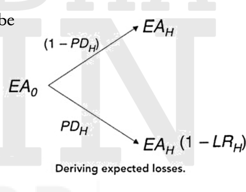
• The expected loss experienced at time \(H(EL_H\), is the difference between the promised exposure amount \(EA_H\) at that time (including all promised interest payments) and the amount that the bank can expect to receive at that time, given that, with a certain probability of default \(PD_H\) between time 0 and H, a loss (\(EA_H\) · \(LR_H\)) will be experienced.
• The expected amount lost (𝐸𝐿) in the event of a default can be defined based on the figure.

Hence,
\( EL_H = EA_H – \left[(1 – PD_H) \cdot EA_H + PD_H \cdot \left(EA_H \cdot (1 – LR_H)\right)\right] = PD_H \cdot EA_H \cdot LR_H \)

Microsoft PowerPoint – CR 3 – Capital Structurie in Banks

where
\(PD_H\) = Probability of default up to time H (horizon)
\(EA_H\)= Exposure amount at time H
\(LR_H\) = Loss rate experienced at time H
\(E(·)\) = Expected Value of (·)

Expected Losses (EL)

Therefore, EL is the product of its three determining components,

• Probability of default (PD): This probability determines whether a counterparty or client goes into default over a predetermined period of time. Although the probability of default can be calculated for any period of time, probabilities are generally estimated at an annual horizon. However, 𝑃𝐷 can and does change over time. A counterparty’s 𝑃𝐷 in the second year of a loan is typically higher than its 𝑃𝐷 in the first year. This behavior can be modeled by using so-called migration or transition matrices. Since these matrices are based on the Markov property, they can be used to derive multiperiod 𝑃𝐷𝑠 – both cumulative and marginal default probabilities.
• Exposure amount (EA): The exposure amount 𝐸𝐴, for the purposes of the 𝐸𝐿 calculation, is the expected amount of the bank’s credit exposure to a customer or counterparty at the time of default. This amount includes all outstanding payments (including interest) at that time. These overall outstanding’s can often be very different from the outstanding’s at the initiation of the credit. This is especially true for the credit risk of derivative transactions (such as swaps), where the quantification of 𝐸𝐴 can be difficult and subject to Monte Carlo simulation.
• Loss rate (LR): When a borrower defaults, the bank does not necessarily lose the full amount of the loan. 𝐿𝑅 represents the ratio of actual losses incurred at the time of default (including all costs associated with the collection and sale of collateral) to 𝐸𝐴. 𝐿𝑅 is, therefore, largely a function of collateral. Uncollateralized, unsecured loans typically have much higher ultimate losses than do collateralized or secured loans.

𝑃𝐷 is a borrower-specific estimate that is typically linked to the borrower’s risk rating, that is, estimated independently of the specifics of the credit facility such as collateral and/or exposure structure. 𝐸𝐴 and 𝐿𝑅 reflect and model the product specifics of a borrower’s liability.

• 𝐸𝐿 due to transfer or country risk can be modeled similarly to this approach and has basically the same three components (𝑃𝐷 of the country, 𝐸𝐴, and 𝐿𝑅 due to country risk). However, there are some more specific aspects to consider. For instance, since a borrower can default due to counterparty and country risk at the same time, one would need to adjust for the “overlap” because the bank can only lose its money once.

• By definition, 𝐸𝐿 does not itself constitute risk. If losses always equaled their expected levels, there would be no uncertainty, and there would be no economic rationale to hold capital against credit risk. Risk arises from the (unexpected) variation in loss levels – which for credit risk is due to unexpected losses (𝑈𝐿). Unexpected loss is the standard deviation of credit losses, and can be calculated at the transaction and portfolio level. Unexpected loss is the primary driver of the amount of economic capital required for credit risk.
• Unexpected loss is translated into economic capital for credit risk in three steps
  • First, the standalone unexpected loss is calculated.
  • Then, the contribution of the standalone 𝑈𝐿 to the 𝑈𝐿 of the bank portfolio is determined.
  • Finally, this unexpected loss contribution (𝑈𝐿𝐶) is translated into economic capital by determining the distance between 𝐸𝐿 and the confidence level to which the portfolio is intended to be backed by economic capital
• Just like 𝐸𝐿, these unexpected losses (𝑈𝐿) are an integral part of the business of lending and stem from the (unexpected) occurrence of defaults and (unexpected) credit migration.

Unexpected Losses (UL-Standalone)

• The 𝑈𝐿𝑠 cannot be anticipated and hence cannot be adequately priced for in a loan’s interest rate. They require a cushion of economic capital, which needs to be differentiated by the risk characteristics of a specific loan.
• 𝑈𝐿, in statistical terms, is the standard deviation of actual credit losses around the expected loss average (𝐸𝐿). The 𝑈𝐿 of a specific loan on a standalone basis (i.e., ignoring diversification effects) can be derived from the components of 𝐸𝐿. Just as 𝐸𝐿 is calculated as the mean of a distribution, 𝑈𝐿 is calculated as the standard deviation of the same distribution.
• For an individual loan, 𝑃𝐷 is (by definition) independent of the 𝐸𝐴 and the 𝐿𝑅, because default is a binary event. Moreover, in most situations, 𝐸𝐴 and the 𝐿𝑅 can be viewed as being independent. Under these assumptions, unexpected loss can be derived as

\(UL = EA \cdot \sqrt{PD \cdot \sigma_{LR}^2 + LR^2 \cdot \sigma_{PD}^2}\)

where
\(\sigma_{LR}\) = Standard deviation of the loss rate 𝐿𝑅
\(\sigma_{PD}\) = Standard deviation of the default probability 𝑃𝐷

• 𝑈𝐿 is dependent on 𝑃𝐷, 𝐿𝑅, and their corresponding variances, \(\sigma_{LR}^2\) and \(\sigma_{PD}^2\) . If there were no uncertainty in the default event and no uncertainty about the recovery rate, both variances would be equal to zero, and hence 𝑈𝐿 would also be equal to zero, indicating that there would be no credit risk. For simplicity, the time index has been ignored in this derivation. But all parameters are estimated, as was done previously, at time 𝐻.
• Since default is a Bernoulli variable with a binomial distribution: \(\sigma_{PD}^2 = PD \cdot (1 – PD)\)
• Since it is typically difficult in practice to measure the variance of the loss rate \(\sigma_{LR}^2\) due to the lack of sufficient historical data, a reasonable distribution will have to be assumed in most cases for the variations in the loss rate. Unfortunately, unlike the distribution for 𝑃𝐷, the loss rate distribution can take a number of shapes, which result in different equations for the variance of 𝐿𝑅. Possible candidates are the binomial, the uniform, or the normal distribution.
• The binomial distribution overstates the variance of 𝐿𝑅 (when a customer defaults, either all of the exposure amount is lost or nothing), The uniform distribution assumes that all defaulted borrowers would have the same probability of losing anywhere between 0% and 100%.
• The most reasonable assumption is the normal distribution, because of the lack of better knowledge in most cases. The shape of this assumed normal distribution should take into account the empirical fact that some customers lose almost nothing, that is, almost fully recover, and it is very unlikely that all of the money is lost during the work-out process.
• Like EL, 𝑈𝐿 can also be calculated for various time periods and for rolling time windows across time. By convention, almost always one-year intervals are used. Hence, all measures of volatility need to be annualized to allow comparisons among different products and business units. Again, the same methodology can be applied to derive the 𝑈𝐿 resulting from country risk using the three components of country 𝐸𝐿.

Unexpected Loss Contribution (ULC)

• Credit risk cannot be completely eliminated by hedging it through the securities markets like market risk. Even credit derivatives and asset securitizations can only shift credit risk to other market players. These actions will not eliminate the downside risk associated with lending. However, they can transfer credit risk to the market participant best suited to bear it, because the only way to reduce credit risk is by holding it in a well-diversified portfolio (of other credit risks). Therefore, it is important to consider credit risk in a portfolio context.
• The expected loss of a portfolio of credits is straightforward to calculate because 𝐸𝐿 is linear and additive. Therefore:
  \( EL_P = \sum_{i=1}^{n} EL_i = \sum_{i=1}^{n} EA_i \cdot PD_i \cdot LR_i \)
• where
• \( EL_P\) = Expected loss of a portfolio of n credits.
• However, when measuring unexpected loss at the portfolio level, the effects of diversification should be considered, because only the contribution of an asset to the overall portfolio risk matters in a portfolio context. In its most general form, the unexpected loss of a portfolio can be defined as:

\( UL_P = \sqrt{\sum_{i=1}^{n} \sum_{j=1}^{n} \rho_{ij} UL_i UL_j} \)

where
\(\rho_{ij}\) = Correlation between default of asset 𝑖 and asset 𝑗 over the same predetermined period
\(𝑈𝐿_i\) Unexpected Loss of the \(𝑖^{th}\) credit asset

• Therefore, considering a loan at the portfolio level, the contribution of a single 𝑈𝐿, to the overall portfolio risk is a function of:
  • The loan’s expected loss (𝐸𝐿), because default probability (𝑃𝐷), loss rate (𝐿𝑅), and exposure amount (𝐸𝐴) all enter the 𝑈𝐿-equation
  • The correlation of the exposure to the rest of the portfolio
• The marginal impact of the inclusion of this loan on the overall credit portfolio risk can be calculated as \( ULMC_i = \left( \sum_{j=1}^{n} UL_j \rho_{ij} \right) \frac{1}{UL_P} \)

where
\(𝑈𝐿𝑀𝐶_i\), is the marginal contribution of loan 𝑖 to the overall portfolio unexpected loss.

In the above formula, the marginal contribution only depends on the (𝑈𝐿−) weights of the different loans in the portfolio, not on the size of the portfolio itself.

The marginal contribution of each loan is constant if the weights of each loan in the portfolio are held constant, which gives

\( UL_{Port} \equiv \sum_{i=1}^{n} ULMC_i \cdot UL_i \)

Therefore, the portfolio 𝑈𝐿 can be viewed to split into 𝑛 components, each of which corresponds to the marginal loss volatility contribution of each loan multiplied by its standalone loss volatility. Hence, the total contribution to the portfolio’s 𝑈𝐿 can be defined as:

\( ULC_i = ULMC_i \cdot UL_i = \left( \sum_{j=1}^{n} UL_j \rho_{ij} \right) \times \frac{1}{UL_p} \times UL_i \)

• 𝑈𝐿𝐶 has the important property that the sum of the 𝑈𝐿𝐶s of all loans will equal the portfolio level 𝑈𝐿 (i.e., the sum of the parts equals the whole, which is exactly the intended result):

\( \sum_{i=1}^{n} ULC_i = UL_p \)

• Assuming now that the portfolio consists of 𝑛 loans that have approximately the same characteristics and size (1/n), and \( \rho_{ij} = \rho = \text{constant} \) (for all \( i \neq j \) ), it can be derived that

\( UL_P = UL_i \sqrt{n + \rho(n^2 – n)} \)

• Using the assumption of similar credits within the portfolio previously described,

\( ULC_i = \frac{UL_P}{n} = \frac{1}{n} UL_i \sqrt{n + \rho(n^2 – n)} = UL_i \sqrt{\frac{1}{n} + \rho \left(1 – \frac{1}{n} \right)} \)

which reduces for large 𝑛 to: \( ULC_i = UL_i \cdot \rho \)

• Hence

\[ \sqrt{\rho} = \frac{\sum_{i=1}^{n} UL_i \cdot \rho_{ij}}{UL_P} \]

which clearly shows that 𝜌 is the (weighted) average correlation between loans in the portfolio (as was assumed above).

• This derivation provides some important insights
  • To estimate the portfolio 𝑈𝐿, [n(n-1)]/2 pairwise default correlations would be required. Given that typical loan portfolios contain many thousand credits, this is impossible to do. Additionally, default correlations are very difficult, if not impossible, to observe.
  • The equation to calculate 𝑈𝐿𝐶 ignores the fact that loans are of different sizes and show different correlations (e.g., by industry, geography, etc.). Therefore, the equation does not reveal potential concentrations in the credit portfolio. But banks try to avoid exactly these concentrations. It is easy to show that the equation can be decomposed for various segments of the portfolio so that, for example, default correlations between various industries or even of a single credit can be included. Using this approach (instead of the impractical “full-blown” approach), allows banks to quantify exactly what they have done by intuition, prudent lending policies, and guidelines for a very long time.
  • Default correlations are small, but positive. Therefore, and as indicated previously, there are considerable benefits to diversification in credit portfolios.
  • Overall, the analytical approach is very cumbersome and prone to estimation errors and problems. To avoid these difficulties, banks now use numerical procedures to derive more exact and reliable results.
• Viewing the UL of a single credit in the context of a credit portfolio reduces the standalone risk considerably in terms of its risk contribution (ULC).

Economic Capital For Credit Risk

• As defined previously, the amount of economic capital needed is the distance between the expected outcome and the unexpected (negative) outcome at a certain confidence level. The unexpected outcomes at the portfolio level are driven by , the estimated volatility around the expected loss. Knowing the shape of the loss distribution, \(EL_P\), and \(UL_P\), one can estimate the distance between the expected outcome and the chosen confidence level as a multiplier (often labeled as capital multiplier, or CM ) of \(UL_p\), as shown in this figure.

img

• Since the sum of \(ULC_is\) equals \(UL_p\), the necessary economic capital at the single transaction level can be attributed as follows:
• Therefore:

\[ \text{Economic Capital}_P = UL_P \times CM \]

\[ \text{Economic Capital}_i = ULC_i \times CM \]

that is, the required economic capital at the single credit transaction level is directly proportional to its contribution to the overall portfolio credit risk.

• The crucial task in estimating economic capital is, therefore, the choice of the probability distribution, because we are only interested in the tail of this distribution. Credit risks are not normally distributed but highly skewed because, as mentioned previously, the upward potential is limited to receiving at maximum the promised payments and only in very rare events to losing a lot of money.
• One distribution often recommended and suitable for this practical purpose is the beta distribution. This kind of distribution is especially useful in modeling a random variable that varies between 0 and 𝑐 (> 0). And, in modeling credit events, losses can vary between 0 and 100%, so that 𝑐 = 1.55 The beta distribution is extremely flexible in the shapes of the distribution it can accommodate.
• By specifying the parameters 𝛼 and 𝛽, the shape of the beta distribution can be determined. It can be shown that if 𝛼 = 𝛽, the beta distribution is symmetric and that when 0 <c < 1, then the mean of the beta distribution equals:

\[ \mu = \frac{\alpha}{\alpha + \beta} \]

and that the variance equals:

\[ \sigma^2 = UL^2_P = \frac{\alpha \beta}{(\alpha + \beta)^2 \cdot (\alpha + \beta + 1)}\]

• The form of the beta distribution is fully characterized by two parameters: \(EL_P\) and \(UL_P\). However, the difficulty is fitting the beta distribution exactly to the tail of the risk profile of the credit portfolio. This tail-fitting exercise is best accomplished by combining the analytical (beta distribution) solution with a numerical procedure such as a Monte Carlo simulation.
• To determine the distance between \(El_P\) and the confidence level, it is required to estimate the probability 𝑝 that the negative deviation of the random variable 𝑋 exceeds the confidence level only in 𝛼% of the cases at the time horizon H. , i.e.

\[ p\left(\frac{X_m – EL_P}{UL_P} \leq CM\right) \leq \alpha \]

• (as indicated by the gray shaded area in the previous figure.
• Taking the inverse of the beta function at the chosen confidence level, 𝐶𝑀 can be determined. Obviously, 𝐶𝑀 is dependent on the overall credit quality of the portfolio and the confidence level. At the typically chosen 99.97% confidence level, 𝐶𝑀 is between 7.0 and 7.5, which is far higher than the capital multiples for the normally distributed events in market risk, given the skewness of the loss distribution.
• The derivation of the economic capital cushion for country risk is identical to the previously described derivation.
  • However, country risk is more “lumpy,” that is, the correlations between single transfer events are higher and there are fewer benefits to diversification because there are only a limited number of countries in the world.
  • Additionally, one needs to consider the correlation between country and counterparty events in deriving the overall economic capital amount.

Problems With The Quantification Of Credit Risk

• Despite the beauty and simplicity of the bottom-up (total) risk measurement approach just described, there are a number of caveats that need to be addressed:
  • This approach assumes that credits are illiquid assets. Therefore, it measures only the risk contribution (i.e., the internal “betas”) to the losses of the existing credit portfolio and not the correlation with risk factors as priced in liquid markets. Since the credit risk of bank loans becomes more and more liquid and is traded in the capital markets, a value approach would be more suitable. Such an approach would estimate the expected return and value of the promised payments and would try to model the probability distribution of changes in the value of the loan portfolio to derive the necessary economic capital.
  • This, however, would require modeling the multi-period nature of credits and, hence, the expected and unexpected changes in the credit quality of the borrowers (and their correlations). Even though this can be easily included in the analytical approach, the more precise numerical solutions get very complex and cumbersome. Therefore, almost all of the internal credit risk models used in practice use only a one year estimation horizon.
  • Although this approach considers correlations at a practicable level, that is, within the same risk type, it assumes, when measuring, that all other risk components (such as market and operational risk) are separated and are measured and managed in different departments within the bank.