Introduction

• Heuristically (or non-mathematically),  two types of financial correlations can be defined
• 1. Static
  2. Dynamic
• Static financial correlations measure how two or more financial assets are associated within a  certain time period. Examples are:
• 1. The classic value-at-risk (VaR) model.
  2. The original copula approach for collateralized debt obligations (CDOs).
  3. The binomial default correlation model of Lucas (1995)
• Dynamic financial correlations measure how two or more financial assets move together in  time. Examples are:
• 1. Pairs trading which is a type of statistical arbitrage
  2. The Heston 1993 model
• Correlations behave randomly and unpredictably. Therefore, it is a good idea to model  them as a stochastic process, which are by construction time dependent.

Financial Correlation Risk

• Financial correlation risk is the risk of financial loss due to adverse movements in correlation  between two or more variables. These variables can comprise any financial variables. For  example, the positive correlation between Mexican bonds and Greek bonds can hurt Mexican  bond investors if Greek bond prices decrease, which happened in 2012 during the Greek crisis.  Or the negative correlation between commodity prices and interest rates can hurt commodity  investors if interest rates rise.
• Correlation risk is especially critical in risk management. An increase in the correlation of asset  returns increases the risk of financial loss, which is often measured by the value-at-risk (VaR)  concept. An increase in correlation is typical in a severe systemic crisis. For example, in the  Great Recession from 2007 to 2009, financial assets and financial markets worldwide became  highly correlated. Risk managers who had assets with negative or low correlations in their  portfolios, suddenly witnessed many of them decline together; hence asset correlations  increased sharply.
• Correlation risk can also involve variables that are nonfinancial, such as economic or political  events. For example, the correlation between the increasing sovereign debt and currency value  can hurt an exporter, as occurred in Europe in 2012, where a decreasing euro hurt U.S.  exporters. Geopolitical tensions as, for example, in the Middle East can hurt airline companies  due to increasing oil prices, or a slowing gross domestic product (GDP) in the United States  can hurt Asian and European exporters and investors, since economies and financial markets  are correlated worldwide.

Financial Correlation Risk-CDS Example

• Let’s look at correlation risk via an  example of  a credit default swap (CDS).  A CDS is a financial product in which the  credit risk is transferred from the investor  (or CDS buyer) to a counterparty (CDS  seller). Let’s assume an investor has  invested $1 million in a bond from Spain.  He is now worried about Spain defaulting  and has purchased a credit default swap  from a French bank, BNP Paribas, as  shown in the figure.
  

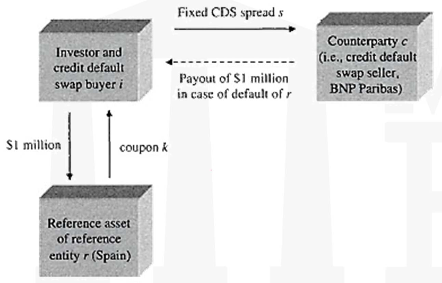
  The investor is protected against a default from Spain, since in case of  default, the  counterparty BNP Paribas will pay the originally invested $1 million to the investor. For  simplicity, let’s assume the recovery rate and accrued interest are zero.

• The value of the CDS, or the fixed CDS spread 𝑠, is mainly determined by the default  probability of the reference entity Spain. However, the spread 𝑠 is also determined by the joint  default correlation of BNP Paribas and Spain. If  the correlation between Spain and BNP  Paribas increases, the present value of  the CDS for the investor will decrease and he will suffer  a paper loss. The worst-case scenario is the joint default of  Spain and BNP Paribas, in which  case the investor will lose his entire investment in the Spanish bond of $1 million. Hence, the  investor is exposed to default correlation risk between the reference asset 𝑟 (Spain) and the  counterparty 𝑐 (BNP Paribas).

• Since both Spain and BNP Paribas are in Europe, it can be assumed that there is a positive  default correlation between the two. In this case, the investor has wrong-way correlation risk.

• Let’s assume the default probability of Spain and BNP Paribas both increase. This means that  the exposure to the reference entity Spain increases (since the CDS has a higher present value  for the investor) and it is more unlikely that the counterparty BNP Paribas can pay the d  insurance.

• The magnitude of the correlation risk is expressed graphically in this figure. It can be observed  that for a correlation of -0.3 and higher, the higher the correlation, the lower the CDS spread.  This is because an increasing 𝜌 means a higher probability of the reference asset and the  counterparty defaulting together. In the extreme case of a perfect correlation of 1, the CDS is worthless. This is because if Spain defaults, so will the insurance seller BNP Paribas.

  
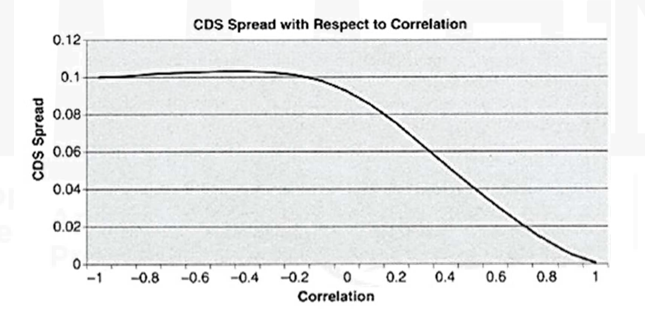
• Also, for a correlation from -1 to about -0.3, the CDS spread increases slightly. This seems  counterintuitive at first. However, an increase in the negative correlation means a higher  probability of either Spain or BNP Paribas defaulting. In the case of Spain defaulting, the CDS  buyer will get compensated by BNP Paribas. However, if the insurance seller BNP Paribas  defaults, the CDS buyer will lose his insurance and will have to repurchase it. This may have to  be done at a higher cost. The cost will be higher if the credit quality of  Spain has decreased  since inception of the original CDS. For example, the CDS spread may have been 3% in the  original CDS, but may have increased to 6% due to a credit deterioration of Spain.
• Hence, it can be said that the dependencies between a variable (here the CDS spread) and  correlation may be non-monotonous; that is, the CDS spread sometimes increases and  sometimes decreases if correlation increases.

Correlation in Different Areas of Finance

• Financial correlations appear in many areas in finance. Five areas are in focus for this topic :
• 1. Investments and correlation
  2. Trading and correlation
  3. Risk management and correlation
  4. The global financial crisis and correlation
  5. Regulation and correlation.
• Naturally, if an entity is exposed to correlation, this means that the entity has correlation risk  (i.e., the risk of a change in the correlation).

Investment and Correlation

• An increase in diversification increases the return/risk ratio. Importantly, high diversification is  related to low correlation. This can be demonstrated with an example. Let’s assume we have a  portfolio of two assets, X and Y, whose performance is given in this table

  Year	Asset X	Asset Y	Return of Asset X	Return of Asset Y
  2008	100	200
  2009	120	230	20.00%	15.00%
  2010	108	460	-10.00%	100.00%
  2011	190	410	75.93%	-10.87%
  2012	160	480	-15.79%	17.07%
  2013	280	380	75.00%	-20.83%
  Average			29.03%	20.07%

• Formulae already done in FRM Part 1 can also be used
  • 
    
    
    
    
    
• If we have a portfolio of these two assets, the portfolio return can be calculated as
  where
  𝑤_x is the weight to asset X,
  and 𝑤_y is the weight to asset Y,
• Also the standard deviation for our two-asset portfolio 𝜌 can be calculated as;
  
  With equal weights, i.e., 𝑤_x = 𝑤_y= 0.5, this example results in 𝜎_ρ = 16.66%. The standard  deviation (or its square, the variance) is interpreted in finance as risk. The higher the standard  deviation, the higher the risk of an asset or a portfolio. Although standard deviation is not a  great measure of risk, but it’s one of  the best we have. A high standard deviation may mean  high upside potential, so it penalizes possible profits! But a high standard deviation naturally  also means high downside risk. In particular, risk-averse investors will not like a high standard deviation, i.e., high fluctuation of their returns.

Trading And Correlation

• If we have a portfolio of these two assets, the portfolio return can be calculated as
  

  where

  𝑤_x is the weight to asset X, and

  𝑤_y is the weight to asset Y,

• Also the standard deviation for our two-asset portfolio 𝜌 can be calculated as

  

  With equal weights, i.e., 𝑤_x  = 𝑤_y= 0.5, this example results in 𝜎_ρ = 16.66%. The standard  deviation (or its square, the variance) is interpreted in finance as risk. The higher the standard deviation, the higher the risk of an asset or a portfolio. Although standard deviation is not a  great measure of risk, but it’s one of the best we have. A high standard deviation may mean  high upside potential, so it penalizes possible profits! But a high standard deviation naturally  also means high downside risk. In particular, risk-averse investors will not like a high standard  deviation, i.e., high fluctuation of their returns.

• In finance, every risk is also an opportunity. Therefore, at every major investment bank and  hedge fund correlation desks exist. The traders try to forecast changes in correlation and  attempt to financially gain from these changes in correlation. Generally, correlation trading  means trading assets whose prices are determined at least in part by the co-movement of one  or more asset in time. Many types of correlation assets exist. Three such assets will be  discussed here :
• 1. Multi-Asset Options
  2. Quanto Option
  3. Correlation Swap

Multi Asset Options

• A popular group of correlation options are multi-asset options, also termed rainbow options or  mountain range options. Many different types are traded. The most popular ones are listed here. 𝑆₁  is the price of asset 1 and 𝑆₂ is the price of asset 2 at option maturity. 𝐾 is the strike price.
  1. Option on the better of two. Payoff = 𝑚𝑎𝑥(𝑆₁, 𝑆₂)
  2. Option on the worse of two. Payoff = 𝑚𝑖𝑛(𝑆₁, 𝑆₂)
  3. Call on the maximum of two. Payoff = 𝑚𝑎𝑥[0, 𝑚𝑎𝑥(𝑆₁, 𝑆₂) — 𝐾]
  4. Exchange option (as a convertible bond). Payoff = 𝑚𝑎𝑥(0, (𝑆₂—𝑆₁))
  5. Spread call option. Payoff = 𝑚𝑎𝑥[0, (𝑆₂ — 𝑆₁) — 𝐾]
  6. Option on the better of two or cash. Payoff = 𝑚𝑎𝑥(𝑆₁, 𝑆₂, 𝑐𝑎𝑠ℎ)
  7. Dual-strike call option. Payoff  = 𝑚𝑎𝑥(0, 𝑆₁   —  𝐾₁, 𝑆₂   —  𝐾₂)
  8. Portfolio of basket options. Payoff =
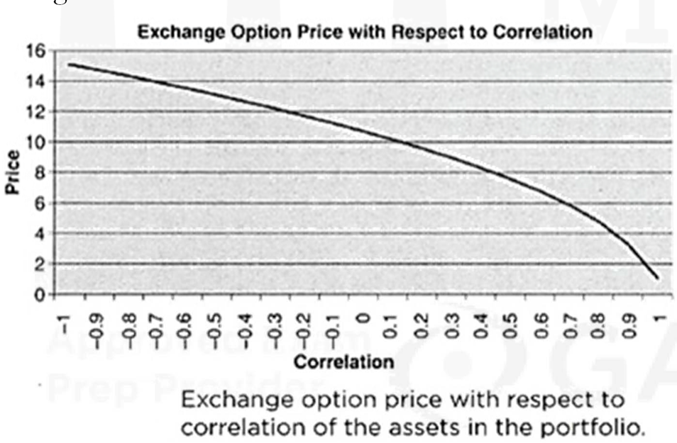
     The prices of these correlation options are highly sensitive to the correlation between the asset  prices 𝑆₁ and 𝑆₂. In the list above, except for the option on the worse of two, the lower the  correlation, the higher the option price. This makes sense since a low, preferable negative  correlation means that if one asset decreases, on average the other increases.
• Let’s look at the evaluation of an exchange option with a payoff of  𝑚𝑎𝑥(0, (𝑆₂—𝑆₁ )). The  payoff shows that the option buyer has the right to give away asset 1 and receive asset 2 at option  maturity. Hence, the option buyer will exercise her right if 𝑆₂ > 𝑆₁ The price of the exchange  option can be derived easily. First the payoff equation is rewritten as
  𝑆₁ × 𝑚𝑎𝑥[0, (𝑆₂/𝑆₁) — 1]. Then implied volatility of 𝑆₂/𝑆₁ is obtained by inputting the  covariance between asset 𝑆₁ and 𝑆₂ to the implied volatility function of the exchange option as
  
  
  Now this 𝜎_E becomes the input to the Black-Scholes-Merton option pricing model
• Importantly, the exchange option price is highly sensitive to the correlation between the asset  prices 𝑆1 and 𝑆2 as seen in this figure, in which the strong impact of the correlation on the  exchange option price is observed. The price is close to 0 for high correlation and $15.08 for a  negative correlation of -1.
  

Quanto Option

• Quanto option allows a domestic investor to exchange his potential option payoff in a foreign currency back into his home currency at a fixed exchange rate. A Quanto option therefore  protects an investor against currency risk. For example, an American believes the Nikkei will  increase, but she is worried about a decreasing yen, which would reduce or eliminate her profits  from the Nikkei call option. The investor can buy a Quanto call on the Nikkei, with the yen  payoff being converted into dollars at a fixed (usually the spot) exchange rate.
• The amount that is re-exchanged to the home currency is unknown, because it depends on the future payoff of the option. Therefore the financial institution that sells a Quanto call does not  know two things:
• 1. How deep in the money the call will be, i.e., which yen amount has to be converted into  dollars.
  2. The exchange rate at option maturity at which the stochastic yen payoff will be converted  into dollars.
• The correlation between the above two i.e. between price of the underlying 𝑆′ and the  exchange rate 𝑋, significantly influences the Quanto call option price.
• Let’s consider a call on the Nikkei 𝑆′ and an exchange rate 𝑋 defined as domestic currency per  unit of foreign currency (so $/1 yen for a domestic American) at maturity.
• If the correlation is positive, an increasing Nikkei will also mean an increasing yen. That is  favorable for the call seller. She has to settle the payoff, but only needs a small yen amount to  achieve the dollar payment. Therefore, the more positive the correlation coefficient, the lower the  price for the Quanto option. If the correlation coefficient is negative, the opposite applies: If the  Nikkei increases, the yen decreases in value. Therefore, more yen are needed to meet the dollar  payment. As a consequence, the lower the correlation coefficient, the more expensive the Quanto  option. Hence, we have a negative relationship between the option price and correlation.
• Quanto options can be conveniently priced closed form applying an extension of the Black-Scholes-Merton 1973 model.

Correlation Swap

• The correlation between assets can also be traded directly with a correlation swap.In a correlation swap a fixed (i.e., known) correlation is exchanged with the correlation that will actually occur, called realized or stochastic (i.e., unknown) correlation, as seen in this figure.
  
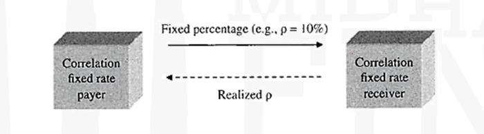
• Paying a fixed rate in a correlation swap is also called buying correlation. This is because the  present value of the correlation swap will increase for the correlation buyer if the realized  correlation increases. Naturally the fixed rate receiver is selling correlation.
• The realized correlation 𝜌 in the previous figure is the correlation between the assets that actually  occurs during the time of the swap. It is calculated as:
  
  where 𝜌_ij is the Pearson correlation between asset 𝑖 and 𝑗,  and 𝑛 is the number of assets in the  portfolio.
  
• The payoff of a correlation swap for the correlation fixed rate payer at maturity is:
  
  where 𝑁 is the notional amount. Let’s look at an example of a correlation swap.

• Correlation swaps can indirectly protect against decreasing stock prices. When stocks decrease,  typically the correlation between the stocks increases. Hence a fixed correlation payer protects  himself indirectly against a stock market decline.

Correlation Swap-Example

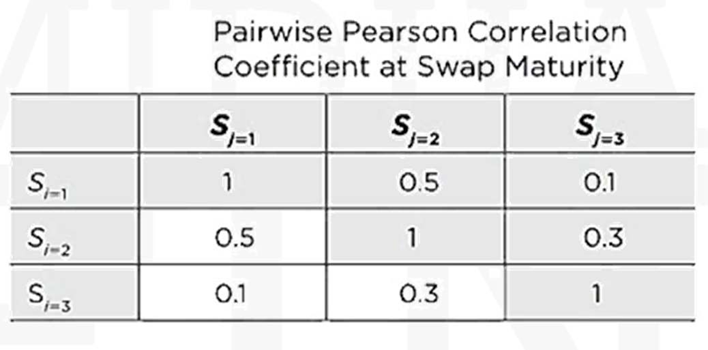
• Consider a correlation swap with three assets, a fixed rate of  10%, a notional amount of $1,000,000, and a 1-year maturity. The realized pair wise correlations of  the log returns at  maturity are as displayed in this table
  

Risk Management And Correlation

• After the global financial crisis from 2007 to 2009, financial markets have become more risk  averse. Commercial banks, investment banks, as well as nonfinancial institutions have increased  their risk management efforts. As in the investment and trading environment, correlation plays a  vital part in risk management.
• Financial risk management is the process of identifying, quantifying, and, if desired, reducing financial risk. The three main types of financial risk 
  
  1. Market risk.
  2. Credit risk.
  3. Operational risk
• Additional types of  risk may include systemic risk, liquidity risk, volatility risk, and correlation  risk. This chapter focuses only on market risk. Market risk consists of four types of risks
  1. Equity risk
  2. Interest rate risk
  3. Currency risk
  4. Commodity risk
• There are several concepts to measure the market risk of a portfolio, such as value-at-risk (VaR),  expected shortfall (ES), enterprise risk management (ERM), and more. VaR is currently (year  2013) the most widely applied risk management measure. Let’s show the impact of  asset  correlation on VaR.
• VaR measures the maximum loss of a portfolio with respect to a certain probability for a certain  time frame. As can be recalled from FRM Part 1, the equation for VaR is
  

  where

  𝑉𝑎𝑅_P is the value-at-risk for portfolio 𝑃

  𝛼 is the critical value of a standard normal distribution corresponding to a certain confidence  level.

  𝑥 is the time horizon for the VaR, typically measured in days

  𝜎_p is the volatility of  the portfolio 𝑃. It can be calculated as where 𝛽_h is the  horizontal 𝛽 vector of invested amounts (price time quantity), 𝛽_v is the vertical 𝛽vector of invested amounts (also price time quantity) and C is the covariance matrix  of the returns of the assets.

Risk Management And Correlation-VaR Example

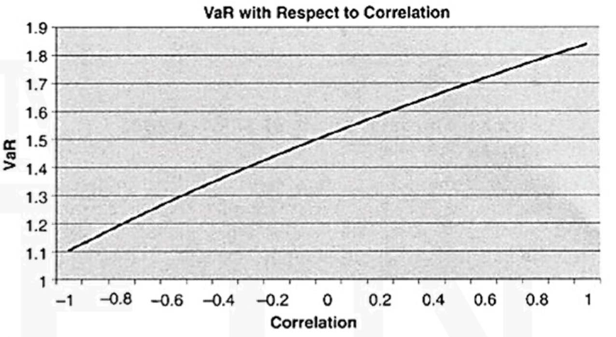
• Let’s now analyze the impact of different  correlations between the asset 1 and asset  2 on VaR. This figure shows the impact.  As expected, we observe from that the  lower the correlation, the lower the risk,  measured by VaR. Preferably the correlation should be negative. In  this  case, if one asset decreases, the other asset  on average increases, hence reducing the  overall risk. The impact of correlation on VaR  is  strong.  For  a  perfect  negative correlation of  -1, VaR is $1.1 million; for  a perfect positive correlation, VaR is close  to $1.9 million. There are no toxic assets,  just toxic people.
  

Global Financial Crisis-Causes

• The global financial crisis of  2007 to 2009 that brought the financial and economic system  worldwide to a standstill had many reasons. Here are the main ones:
• 1. An extremely benign economic and risk environment from 2003 to 2006 with record low  credit spreads, low volatility, and low interest rates.
  2. Increasing risk taking and speculation of traders and investors who tried to benefit in these  presumably calm times. This led to a bubble in virtually every market segment, such as the  housing market, mortgage market (especially the subprime mortgage market), stock  market, and commodity market. In 2007, U.S. investors had borrowed 470% of the U.S.  national income to invest and speculate in the real estate, financial, and commodity  markets.
  3. A new class of structured investment products, such as collateralized debt obligations  (CDOs), CDO squareds, constant-proportion debt obligations (CPDOs), constant-  proportion portfolio insurance (CPPI), as well as new products like options on credit  default swaps (CDSs), credit indexes, and the like.
  4. The new copula correlation model, which was trusted naively by many investors and which could presumably correlate the assets in astructured product. Most CDOs contained 125 assets. Hence there are asset correlation pairs to be quantified and managed.
  5. A moral hazard of  rating agencies, which were paid by the same companies whose assets  they rated. As a consequence, many structured products received AAA ratings and gave the  illusion of little price and default risk.
  6. Risk managers and regulators who lowered their standards in light of the greed and profit  frenzy.

Global Financial Crisis and Correlation

• The first correlation-related crisis occurred in May 2005. General Motors was downgraded to  BB and Ford was downgraded to BB+, so both companies were now in junk status. A  downgrade to junk status typically leads to a sharp bond price decline, since many mutual funds  and pension funds are not allowed to hold junk bonds. Importantly, the correlation of  the  bonds in CDOs that referenced investment grade bonds decreased, since bonds of different  credit qualities are typically lower correlated. This led to huge losses of hedge funds, which had  put on a strategy where they were short the equity tranche of the CDO and long the mezzanine  tranche of the CDO.
  

  This figure shows the dilemma. Hedge funds had  shorted the equity tranche (0% to 3 %) to collect the  high equity tranche spread. They had then presumably  hedged the risk by going long the mezzanine tranche”  (3% to 7%). However, as we can see from this figure,  this hedge is flawed.

  

• • When the correlations of the assets in the CDO decreased, the hedge funds lost on both  positions.
  • 1. The equity tranche spread increased sharply (indicated by the arrow 1 in the previous  figure). Hence the fixed spread that the hedge funds received in the original transaction was  now significantly lower than the current market spread, resulting in a paper loss.
    2. In addition, the hedge funds lost on their long mezzanine tranche positions, since a lower  correlation lowers the mezzanine tranche spread; (indicated by the arrow 2 in the previous  figure). Hence the spread that the hedge funds paid in the original transactions was now  higher than the market spread, resulting in another paper loss.
  • As a result of the huge losses, several hedge funds, such as Marin Capital, Aman Capital, and  Baily Coates Cromwell, filed for bankruptcy. It is important to point out that the losses resulted  from a lack of understanding of the correlation properties of the tranches in the CDO. The  CDOs themselves can hardly be blamed or be called toxic for their correlation properties.
  • From 2003 to 2006 the CDO market, mainly referencing residential mortgages, had exploded,  increasing from $64 billion to $455 billion. To fuel the CDOs, more and more questionable  subprime mortgages were given, named NINJA loans, standing for “no income, no job or  assets.” When housing prices started leveling off in 2006, the first mortgages started to default.  In 2007 more and more mortgages defaulted, finally leading to a real estate market collapse.  With it the huge CDO market collapsed, leading to the stock market and commodity market  crash and a freeze in the credit markets. The financial crisis spread to the world economies,  creating a global severe recession, now called the Great Recession.
  • In a systemic crash like this, naturally many types of correlations From 2007 to 2009, default  correlations of the mortgages in the CDOs increased. This actually helped equity tranche  investors, because If default correlations increase, the equity tranche spread decreases, leading  to an increase in the value of  the equity tranche. However, this increase was overcompensated  by a strong increase in default probability of the mortgages. As a consequence, tranche spreads  increased sharply, resulting in huge losses for the equity tranche investors as well as investors in  the other tranches.
  • Correlations between the tranches of the CDOs also increased during the crisis. This had a  devastating effect on the super-senior tranches. In normal times, these tranches were considered  extremely safe since (1) they were AAA rated and (2) they were protected by the lower tranches.  But with the increased tranche correlation and the generally deteriorating credit market, these  super senior tranches were suddenly considered risky and lost up to 20% of  their value. To  make things worse, many investors had leveraged the super-senior tranches, termed leveraged  super-senior (LSS) tranches, to receive a higher spread.
  • The credit default swap (CDS) market also exploded from its beginnings in the mid-1990s from  about $8 trillion in 2004 to almost $60 trillion in 2007. CDSs are typically used as insurance to  protect against default of  a debtor. CDSs, though, can also be used as speculative instruments.  For example, the CDS seller (i.e., the insurance seller) hopes that the insured event (e.g., default  of a company or credit deterioration of the company) will not occur. In this case the CDS seller  keeps the CDS spread (i.e., the insurance premium) as income, as American International  Group (AIG) tried to do in the crisis. A CDS buyer who does not own the underlying asset is  speculating on the credit deterioration of  the underlying asset, just like a naked put option  holder speculates on the decline of the underlying asset.

  Regulation and Correlation

  • Correlations are critical inputs in regulatory frameworks such as the Basel accords, especially in regulations for market risk and credit risk. Basel I, implemented in 1988; Basel II, implemented in 2006; and Basel III, which is currently being implemented, are regulatory guidelines to ensure the stability of the banking system. None of the Basel accords has legal authority. However, most countries have created legislation to enforce the Basel accords for their banks.
  • The objective of the Basel accords is to “provide incentives for banks to enhance their risk measurement and management systems” and “to contribute to a higher level of safety and soundness in the banking system.” In particular, Basel III addresses the deficiencies of the banking system during the financial crisis of 2007 to 2009. Basel III introduces many new ratios to ensure liquidity and adequate leverage of banks. In addition, new correlation models will be implemented that deal with double defaults in insured risk transactions. Correlated defaults in a multi-asset portfolio quantified with the Gaussian copula, correlations in derivatives transactions termed credit value adjustment (CVA), and correlations in what is called wrong-way risk (WWR) have been discussed.

  Correlation and Market Risk

  • Correlation risk is an integral part of market risk. Market risk is comprised of  equity risk,  interest rate risk, currency risk, and commodity risk. Market risk is typically measured with the  value-at-risk (VaR) concept. VaR has a covariance matrix of the assets in the portfolio as an  input. So market risk implicitly incorporates correlation risk, i.e., the risk that the correlations  in the covariance matrix change.
  • Market risk is also quantified with expected shortfall (ES), also termed conditional VaR or tail  risk. Expected shortfall measures market risk for extreme events, typically for the worst 0.1 %,  1%, or 5% of possible future scenarios. A rigorous valuation of expected shortfall naturally  includes the correlation between the asset returns in the portfolio, as VaR does.

  Correlation and Credit Risk

  • Correlation risk is also a critical part of credit risk. Credit risk is comprised of
    1. Migration risk
    2. Default risk
  • Migration risk is the risk that the credit quality of a debtor decreases, i.e., migrates to a lower  credit state. A lower credit state typically results in a lower asset price, so a paper loss for the  creditor. The effect of  correlation risk of  an investor who has hedged his bond exposure with  a CDS has already been examined earlier. The higher the correlation, the higher the CDS paper  loss for the investor and, importantly, the higher the probability of a total loss of  the  investment.
  • Default risk relates to the degree to which defaults occur together (i.e., default correlation) and  is critical for financial lenders such as commercial banks, credit unions, mortgage lenders, and  trusts, which give many types of  loans to companies and individuals. Default correlations are  also critical for insurance companies, which are exposed to credit risk of numerous debtors.  Naturally, a low default correlation of debtors is desired to diversify the credit risk.
  • This table shows the default correlation from 1981 to 2001 of 6,907 companies, of which 674 defaulted.

    	Auto	Cons	Ener	Fin	Build	Chem	HiTech	Insur	Leis	Tele	Trans	Util
    Auto	3.80%	1.30%	1.20%	0.40%	1.10%	1.60%	2.80%	-0.50%	1.00%	3.90%	1.30%	0.50%
    Cons	1.30%	2.80%	-1.40%	1.20%	2.80%	1.60%	1.80%	1.10%	1.30%	3.20%	1.30%	1.90%
    Ener	1.20%	-1.40%	6.40%	-2.50%	-0.50%	0.40%	-0.10%	-1.60%	-1.00%	-1.40%	-0.10%	0.70%
    Fin	0.40%	1.20%	-2.50%	5.20%	2.60%	0.10%	2.30%	3.00%	1.60%	3.70%	1.50%	4.50%
    Build	1.10%	2.80%	-0.50%	2.60%	6.10%	1.20%	2.30%	1.80%	2.30%	6.50%	4.20%	1.30%
    Chem	1.60%	1.60%	0.40%	0.10%	1.20%	3.20%	1.40%	-1.10%	1.10%	2.80%	1.10%	1.00%
    HiTech	2.80%	1.80%	-0.10%	0.40%	2.30%	1.40%	3.30%	0.00%	1.10%	4.70%	1.10%	1.00%
    Insur	-0.50%	1.10%	-1.60%	3.00%	1.80%	-1.10%	0.00%	5.60%	1.20%	-2.60%	2.30%	1.40%
    Leis	1.00%	1.30%	-1.00%	1.60%	2.30%	1.10%	1.40%	1.20%	2.30%	4.00%	2.30%	0.60%
    Tele	3.90%	3.20%	-1.40%	3.70%	6.50%	2.80%	4.70%	-2.60%	4.00%	10.70%	3.20%	1.00%
    Trans	1.30%	2.70%	-0.10%	1.50%	4.20%	1.10%	1.10%	2.30%	2.30%	3.20%	4.30%	3.20%
    Util	0.50%	1.90%	0.70%	4.50%	1.30%	1.00%	1.00%	1.40%	0.60%	-0.80%	-0.20%	9.40%

  • From the previous table it can be observed that
  • 1. Default correlations between industries are mostly positive with the exception of  the  energy sector. This sector is typically viewed as a recession-resistant, stable sector with little  or no correlation to other sectors.
    2. Default correlation within sectors is higher than between sectors. This suggests that  systematic factors (e.g., a recession or structural weakness such as the general decline of a  sector) have a greater impact on defaults than do idiosyncratic factors. Hence if General  Motors defaults, it is more likely that Ford will default, rather than Ford benefiting from  the default of its rival.

       Since the intra-sector default correlations are higher than inter-sector default correlations, a  lender is advised to have a sector-diversified loan portfolio to reduce default correlation risk.

  • Defaults are binomial events, either default or no default. So principally, a simple correlation model such as the binomial model of Lucas (1995) can be used to analyze them. However, they can also be analyzed in more detail by looking at term structure of defaults. Let’s assume a creditor has given loans to two debtors. One debtor is A rated, and one is CC rated. A historical default term structure of these bonds is displayed in this table
    Term Structure of Default probabilities for an A-Rated Bond and a CC-Rated Bond in 2022

    	Year
    	1	2	3	4	5	6	7	8	9	10
    A	0.02%	0.07%	0.13%	0.14%	0.15%	0.17%	0.18%	0.21%	0.24%	0.25%
    CC	23.83%	13.29%	10.31%	7.62%	5.04%	5.13%	4.04%	4.62%	2.62%	2.04%

   

  	Yea
  	1	2	3	4	5	6	7	8	9	10
  A	0.02%	0.07%	0.13%	0.14%	0.15%	0.17%	0.18%	0.21%	0.24%	0.25%
  CC	23.83%	13.29%	10.31%	7.62%	5.04%	5.13%	4.04%	4.62%	2.62%	2.04%

  

  • For most investment grade bonds, the term structure of default probabilities increases in time. This is because the longer the time horizon, the higher the probability of adverse internal events such as mismanagement, or adverse external events such as increased competition or a recession. For bonds in distress, however, the default term structure is typically inverse. This is because for a distressed company the immediate future is critical. If the company survives the coming problematic years, the probability of default decreases.
  • For a creditor, the default correlation of her debtors is critical. As mentioned, a creditor will benefit from a low default correlation of her debtors, which spreads the default correlation risk.

  Correlation Risk and Systemic Risk

  • Systemic Risk is the risk of a financial market or an entire financial system collapsing. An example of systemic risk is the collapse of the entire credit market in 2008. At the height of the crisis in September 2008, when Lehman Brothers filed for bankruptcy, the credit markets were virtually frozen with essentially no lending activities. Even as the Federal Reserve guaranteed interbank loans, lending resumed only very gradually and slowly.
  • The stock market crash starting in October 2007 with the Dow Jones Industrial Average at  14,093 points and then falling by 53.54% to 6,547 points by March 2009 is also a systemic market collapse. All but one of the Dow 30 stocks had declined. Walmart was the lone Dow stock that was up during the crisis. Of the S&P 500 stocks, 489 declined during this time frame. Consumer staples sector (which provides such basic necessities as food and household items) fared well during the crisis. The educational sector also typically thrives in a crisis, since many unemployed seek to further their education.
  • Importantly, systemic financial failures such as the one from 2007 to 2009 typically spread to the economy, with a decreasing GDP, increasing unemployment, and therefore a decrease in the standard of living.
  • Systemic risk and correlation risk are highly dependent. Since a systemic decline in stocks involves almost the entire stock market, correlations between the stocks increase sharply. This figure shows the relationship between the percentage change of the Dow Jones Industrial Average, (Dow), and the correlation between the stocks in the Dow before the crisis from May  2004 to October 2007 and during the crisis from October 2007 to March 2009.
    
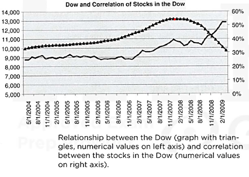
  • To construct this graph, daily closing prices of all 30 stocks in the Dow have been downloaded and put into monthly bins. Then monthly 30 × 30 correlation matrices have been derived using the Pearson correlation measure and the matrices have been averaged. After that, the graph has been smoothened by taking the one-year moving average.

  Correlation Risk and Concentration Risk

  • Concentration risk is a fairly new risk category. Although, it is not yet uniquely defined, but a stable definition can be –
    Concentration risk is the risk of financial loss due to a concentrated exposure to a particular group of counterparties.
  • Concentration risk can be quantified with the concentration ratio. For example, if a creditor has  10 loans of equal size, the concentration ratio would be ^1⁄₁₀ = 0.1. If a creditor has only one loan to one counterparty, the concentration ratio would be 1. Naturally, the lower the concentration ratio, the more diversified is the default risk of the creditor, assuming the default correlation between the counterparties is smaller than 1.
  • The counterparties can be categorized into groups, for example sectors, and then sector concentration risk can be analyzed. The higher the number of different sectors a creditor has lent to, the higher is the sector diversification. High sector diversification reduces default risk, since intra-sector defaults are more highly correlated than counterparties in different sectors, as seen in an earlier table.

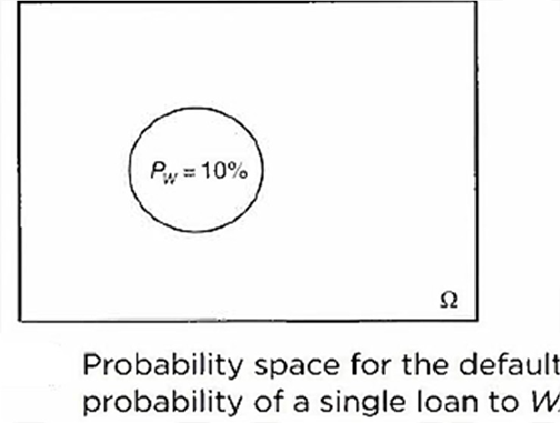
  CASE A

  • The commercial bank 𝐶 has lent $10,000,000 to a single company, 𝑊. So 𝐶’s concentration ratio is 1. Let’s assume company 𝑊 has a default probability (𝑃_w) of 10%. Hence the expected loss (EL) for bank C is $10,000,000 × 0.1 = $1,000,000
    

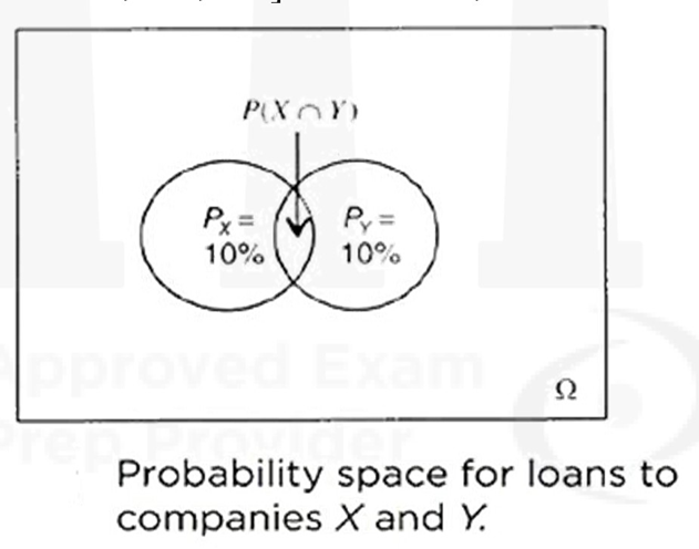
  CASE B

  • The commercial bank 𝐶 has lent $5,000,000 to company 𝑋 and $5,000,000 to company 𝑌. Let’s assume both 𝑋 and 𝑌 have a 10% default probability. So C’s concentration ratio is reduced to ½. If the default correlation between 𝑋 and 𝑌 is bigger than 0 and smaller than 1, the probability of the worst-case scenario [i.e., the default probability of 𝑋 and 𝑌 together, (or 𝑃(𝑋 ∩ 𝑌)), with a loss of $1,000,000] is reduced, as seen in this figure
  • The exact joint default probability 𝑃(𝑋 ∩ 𝑌) depends on the correlation model and correlation parameter values, which will be discussed in later chapters. For any model, though, if default correlation between X and Y is 1, then there is no benefit from the lower concentration ratio. The probability space would have the form as in the previous figure.
    
  • A decreasing concentration ratio is closely related to a decreasing correlation coefficient. Let’s show this. The defaults of companies X and Y are expressed as two binomial variables, which take the value 1 if in default, and 0 otherwise. The following equation gives the joint probability of default for the two binomial events:
    

    where

    𝜌_KF is the correlation coefficient

    is the standard deviation of the binomially distributed variable 𝑋

    is the standard deviation of the binomially distributed variable 𝑌

  CASE B – EXAMPLE

  • Let’s assume again that the lender 𝐶 has given loans to 𝑋 and 𝑌 of $5,000,000 each. Both 𝑋 and 𝑌 have a default probability of 10%. Hence, the standard deviation for both 𝑋 and 𝑌 is
    

    The default correlation is 𝜌_KF = 1. This means that 𝑋 and 𝑌 cannot default individually. They  can only default together or survive together. The probability that they default together is 10%.  Hence the expected loss is the same as in CASE A:

  • Subcase I –

    The default correlation is 𝜌_KF = 1. This means that 𝑋 and 𝑌 cannot default individually. They  can only default together or survive together. The probability that they default together is 10%. Hence the expected loss is the same as in CASE A:

    𝐸𝐿 = ($5,000,000 + $5,000,000) × 0.1 = $1,000,000

    This can ne verified for the joint probability of two binomial events,

    

    The probability space is graphically the same as CASE A.
  • Subcase II –

    The default correlation is decreased to 𝜌_KF = 0.5. The oint probability becomes

    
  • Subcase III –

    The default correlation is decreased to 𝜌_KF = 0. The oint probability becomes

    
  • In conclusion, the beneficial aspect of a lower concentration ratio is clearly visible, which is  closely related to a lower correlation coefficient. In particular, both a lower concentration ratio  and a lower correlation coefficient reduce the worst-case scenario for a creditor, the joint  probability of default of his debtors.

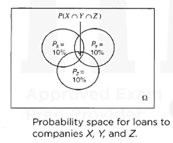
  CASE C

  • If the concentration ratio is further decreased , the probability of  the worse-case scenario (i.e.,  the expected loss of 10%) decreases further. Let’s assume the lender C gives loans to three  companies, X, Y, and Z, of  $3.33 million each. Let’s assume that the default probabilities of  X,  Y, and Z are 10% each. Therefore the concentration ratio decreases to ^1⁄₃. The probabilities are  given in this figure.
    
  • So overall, the benefits of  a lower concentration ratio  are clearly observed. The worst-case scenario, an  expected loss of $1,000,000, reduces with a decreasing  concentration ratio.