
Learning Objectives
- Describe the models that can be estimated using linear regression and differentiate them from those which cannot.
- Interpret the results of an OLS regression with a single explanatory variable.
- Describe the key assumptions of OLS parameter estimation.
- Characterize the properties of OLS estimators and their sampling distributions.
- Construct, apply, and interpret hypothesis tests and confidence intervals for a single regression coefficient in a regression.
- Explain the steps needed to perform a hypothesis test in a linear regression.
- Describe the relationship between a t-statistic, it’s p-value, and a confidence interval.
- Video Lecture
- |
- PDFs
- |
- List of chapters
Chapter Contents
- Introduction
- Regression Analysis in Econometrics – Example
- Linear Regression parameters
- Linearity
- Transformations
- Dummy Variables
- Ordinary Least Squares
- Ordinary Least Squares – Beta Estimator
- Ordinary Least Squares – Alpha Estimator
- Ordinary Least Squares
- Ordinary Least Squares – Example
- Ordinary Least Squares – Result
- Properties of Ols Parameter Estimators
- Properties of Ols Slope Estimator
- properties of Ols Intercept Estimator
- Inference and Hypothesis Testing
Introduction
- Linear regression is a widely applied statistical tool for modeling the relationship between random variables. It has many appealing features that can be adapted to a wide variety of problems. Regression is surprisingly flexible and can describe a wide variety of relationships.
- Dummy variables and interactions are two key tools used when modeling data. These are widely used to build flexible models where parameter values change depending on the value of another variable.
- Ordinary Least Squares (OLS) estimators have a simple moment-like structure and depend on the mean, variance, and covariance of the data. When six key assumptions are satisfied, the parameter estimators are asymptotically normal, and standard inference can be used to test hypotheses.
- There are three key applications of linear regression in finance:
- measuring asset exposure to risk factors,
- hedging, and
- evaluating fund manager performance.
Regression Analysis in Econometrics – Example
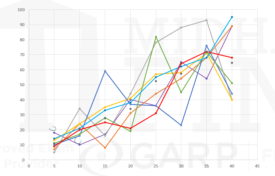
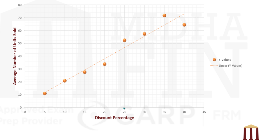
- MidhaKart is an online mobile retailer. It wants to assess the increase in sales with an increase in discount percentage offered by the company.
| Discount Percentage |
Number of units of phones sold (in thousands) | ||||||||
| Phone A | Phone B | Phone C | Phone D | Phone E | Phone F | Phone G | Phone H | Average | |
| 5 | 18 | 7 | 5 | 13 | 10 | 11 | 14 | 9 | 10.875 |
| 10 | 10 | 24 | 34 | 24 | 16 | 17 | 21 | 20 | 20.75 |
| 15 | 17 | 8 | 16 | 35 | 59 | 28 | 33 | 25 | 27.625 |
Linear Regression parameters
- Linear regression assumes a linear relationship between an explanatory variable 𝑋 and a dependent variable 𝑌 so that:
where :
- β, the slope or the regression coefficient, measures the sensitivity of Y to changes in X;
- α, the intercept, is a constant; and
- ϵ, the shock/innovation/error, represents a component in Y that cannot be explained by X. This shock is assumed to have mean 0 so that
- The presence of the shock is also why statistical analysis is required. If the shock were not present, then Y and X would have a perfect linear relationship and the value of the two parameters could be exactly determined using only basic algebra.
Variable Naming Conventions
| Explained Variable | Explanatory Variable | Shock |
| Left-Hand-Side Variable | Right-Hand-Side Variable | Innovation |
| Dependent Variable | Independent Variable | Noise |
| Regressand | Regressor | Error |
| Disturbance |
Linearity
- Explanatory variables can be continuous, discrete, or functions of one or more variables (e.g., X3 = X1×X2). However, all linear regressions must satisfy three essential restrictions.
- First, the relationship between 𝑌 and the explanatory variables X1,X2, … , Xk must be linear in the unknown coefficients. This means that the term on the right-hand-side of the model must have a single unknown coefficient multiplied by a single explanatory variable.
- Second, the error must be additive. This restriction excludes some models where the variance of the error depends on observed data (e.g., 𝑌 = 𝛼 + 𝛽𝑋 + 𝛾𝑋𝜖).
- Finally, all explanatory variables must be observable. This limitation precludes directly applying linear regression with missing data.
- However, the use of multiple regression (i.e., multiple explanatory variables) can allow some nonlinear relationships to be modeled using linear regression. The multiple regression model includes 𝑘 explanatory variables so that:
- Building models with multiple explanatory variables allows the effect of an explanatory variable to be measured while controlling for other variables known to be related to Y. For example, when assessing the performance of a hedge fund manager, it is common to use between seven and 11 explanatory variables that capture various sources of risk.
- The explanatory variables are not assumed to be independent, and so one variable can be defined as a known nonlinear function of another.
For example, consider
Transformations
- Some model specifications can be transformed so that they satisfy the three requirements for linearity. For example, suppose that Y is an always positive random variable, and that Y, X, and ϵ are related through:
- When interpreting the slope of a transformed relationship, note that the coefficient β measures the effect of a change in the transformation of X on the transformation of Y.
where ϵ is a positive-valued shock.
This specification is not compatible with the requirements of linear regression, because X is raised to an unknown coefficient β and the error 𝜖 is not additive.
However, taking the natural logarithm of both sides of the equation transforms the relationship.
Dummy Variables
- An important class of explanatory variable is known as a dummy. A dummy random variable is binary and only takes the value 0 or 1. Dummies are used to e in).
- A dummy takes the value 1 when the observation has the quality and 0 if it does not. For example, when encoding sectors, the transportation sector dummy is 1 for a firm whose primary business is transportation (e.g., a commercial airline or a bus operator) and 0 for firms outside the industry. Dummies are also commonly constructed as binary transformations of other random variables (e.g., a market direction dummy that encodes the return on the market as 1 if negative and 0 if positive).
- Dummies can be added to models to change the intercept (α) or the slope (β) when the dummy variable takes the value 1.
Ordinary Least Squares
- Consider a basic regression model that includes a single explanatory variable:
- These parameters can be estimated using Ordinary Least Squares (OLS) estimators, which are derived by minimizing the sum of squared deviations. The squared deviations being minimized are between the realizations of the dependent variable Y and their expected values given the respective realizations of X:
- In turn, these estimators minimize the residual sum of squares, which is defined as:
This model has three parameters
α (i.e., the intercept),
β (i.e., the slope), and
σ2 (i.e., the variance of ϵ).
where
argmin denotes argument of the minimum, and all n pairs (xi , yi) are the realizations of X and Y.
In other words, the estimators (i.e., α ̂ and β ̂) are the intercept and slope of a line that best fits the data because it minimizes the squared deviations between the line α ̂+β ̂xi and the realizations of the dependent variable yi .
Ordinary Least Squares – Beta Estimator
- The solution to the minimization problem is
- This ratio can also be rewritten in terms of the correlation and the standard deviations so that
- Note that the estimator β ̂ is only sensible if ∑i=1n(xi – X ̅ )2 > 0, or σX2 > 0, which requires that xi has some variation around its mean. If xi only takes one value, then all points lie along a vertical line and the slope is infinite.
Diving the numerator and denominator by 1⁄n, β ̂ can be shown to be
Ordinary Least Squares – Alpha Estimator
- The regression was given by
- This means that if one of α ̂ or β ̂ is estimated, the other can be calculated easily. To summarize,
For any point that lies exactly on the best fit line, ϵ=0
It turns out that the regression line always passes through the point which denotes the mean of X and the mean of Y, i.e. the point (X ̅,Y ̅)
where
Y ̅and X ̅ are the means of yi and xi , respectively.
Ordinary Least Squares
- The estimators α ̂ and β ̂ are then used to construct the fitted values:
- The residuals are always mean 0 and uncorrelated with Xi. These two properties are consequences of minimizing the sum of squared errors. These residuals are different from the shocks in the model, which are never observed.
- The sample correlation ρxy uniquely determines the direction of the line relating Y and X. It also plays a role in determining the magnitude of the slope.
- Also, the sample standard deviations σ ̂y and σ ̂x scale the correlation in the final determination of the regression coefficient β ̂ . This relationship highlights a useful property of OLS: ρ=0 if and only if β=0.
and the model residuals
Finally, the variance of the shocks is estimated by:
The variance estimator divides by n-2 to account for the two estimated parameters in the model, so that s2 is an unbiased estimator of σ2 (i.e., E[s2] = σ2 ).
Ordinary Least Squares – Example
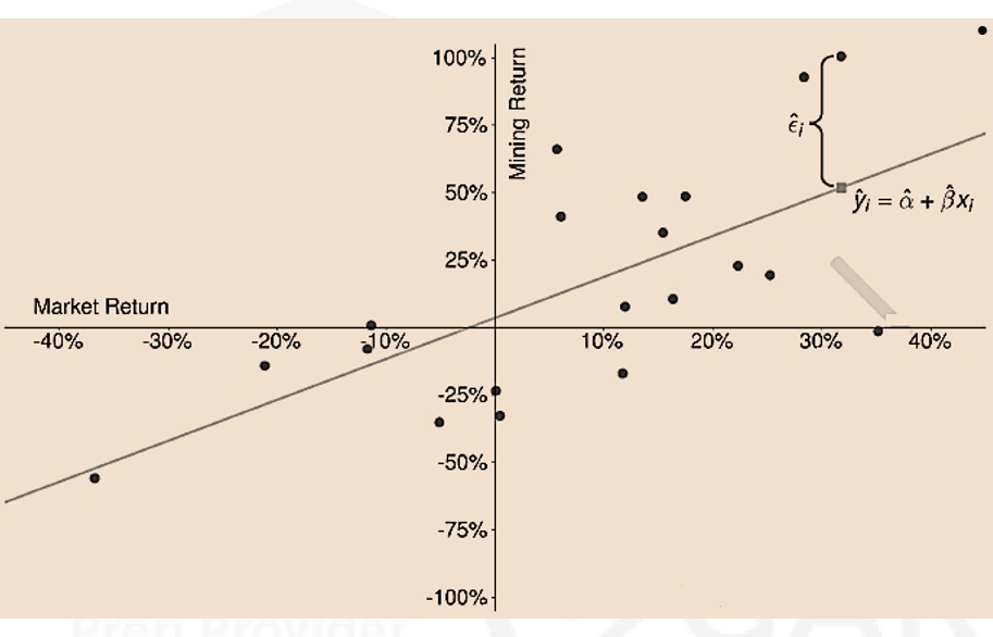
- This figure illustrates the components of a fitted model that regresses the mining sector portfolio returns on the market return for 20-year period between 1999 and 2018. The solid line is the estimated regression line, which minimizes the sum of the squared vertical distances between the observed data and the fitted line.
- The mean annual excess returns of the mining sector (Y) and the market (X) are y ̅= 15.4% and x ̅=7.77%. The covariance matrix for the two annual returns is
- The estimated slope shows that the return on the mining sector portfolio increases by an average of 1.5188% when the market return increases by 1%.
- The estimated intercept indicates that the portfolio returns an average of 3.5987% when the market return is zero.
Ordinary Least Squares – Result
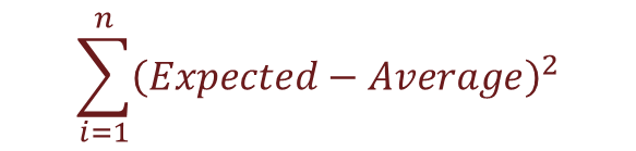
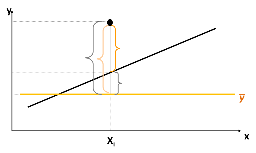
- Explained Sum of Squares
- The explained sum of squares (ESS) is the sum of squared deviations of the predicted values of Yi (i.e. (Yi ) ̂ ), from the average of the Yi’s (i.e. Y ̅).
- Sum of Squared Residuals
- The sum of squared residuals/errors (RSS/SSR) is the sum of squared deviations of the actual (or observed) values of Yi, from the predicted value of Yi (i.e.. (Yi ) ̂).
- Total Sum of Squares
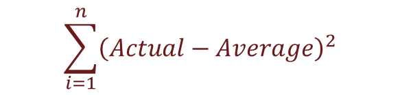
- The total sum of squares (TSS) is the sum of squared deviations of the actual (or observed) values of Yi, from the average of the Yi’s (i.e. Y ̅).
- R2 is the proportion of the variance in the dependent variable that is explained by the (variation in) the independent variable. It is calculated as the ratio of the explained sum of squares to the total sum of squares
- IMPORTANT – For a linear regression with a single regressor
- MidhaKart Example revisited
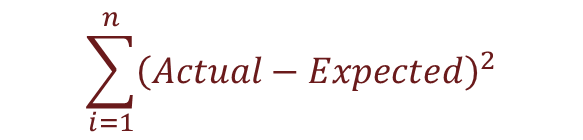
Hence SSR is simply the sum of the squares of the error terms, i.e.
It is important to note that
TSS = ESS+RSS


Since TSS = ESS + RSS ⇒ ESS = TSS – RSS
So R2 can also be written as
Remember that this result is not valid for linear regression with multiple regressors.
Calculations to be done in excel. In the video manual calculation has also been shown.
| Discount Percentage |
Number of sales of the phone (in thousands) | ||||||||
| Phone A | Phone B | Phone C | Phone D | Phone E | Phone F | Phone G | Phone H | Average | |
| 5 | 18 | 7 | 5 | 13 | 10 | 11 | 14 | 9 | 10.875 |
| 10 | 10 | 24 | 34 | 24 | 16 | 17 | 21 | 20 | 20.75 |
| 15 | 17 | 8 | 16 | 35 | 59 | 28 | 33 | 25 | 27.625 |
| 20 | 40 | 31 | 44 | 41 | 37 | 19 | 38 | 21 | 33.875 |
| 25 | 36 | 44 | 78 | 57 | 36 | 82 | 55 | 31 | 52.375 |
| 30 | 65 | 54 | 88 | 58 | 23 | 45 | 62 | 64 | 57.375 |
| 35 | 54 | 68 | 93 | 71 | 76 | 72 | 68 | 72 | 71.75 |
| 40 | 89 | 89 | 40 | 40 | 44 | 51 | 95 | 68 | 64.5 |
Properties of Ols Parameter Estimators
- The derivation of OLS estimators requires only one easy-to-verify assumption – that the variance of X is positive. However, a total of six assumptions are needed to establish conditions that ensure the OLS estimators are interpretable and have desirable statistical properties.
- Shocks Are Mean Zero – Shocks are mean zero conditional on X, so that E[ϵ|X]=0. This property is known as mean independence and it requires that X has no information about the location of ϵ.
- These assumptions come with two meaningful implications.
- First, they imply that the estimators are unbiased.
- The second meaningful implication is that the two estimators are jointly normally distributed.
i) This assumption implies that Corr[ϵ, X]=0
ii) It also implies that the unconditional mean of the errors is zero (E[ϵ]=0).
iii) This assumption is not directly testable as shocks are not observable and the estimated residuals (i.e., ϵ ̂i) are always exactly uncorrelated with the observations of the explanatory variable (i.e., xi). Determining whether this assumption is reasonable requires a careful examination of the data generating process for (Y, X).
iv) Examples of data generating processes where the first assumption is violated –
a)Sample selection bias or survivorship bias
b)Simultaneity bias
c)Omitted variables
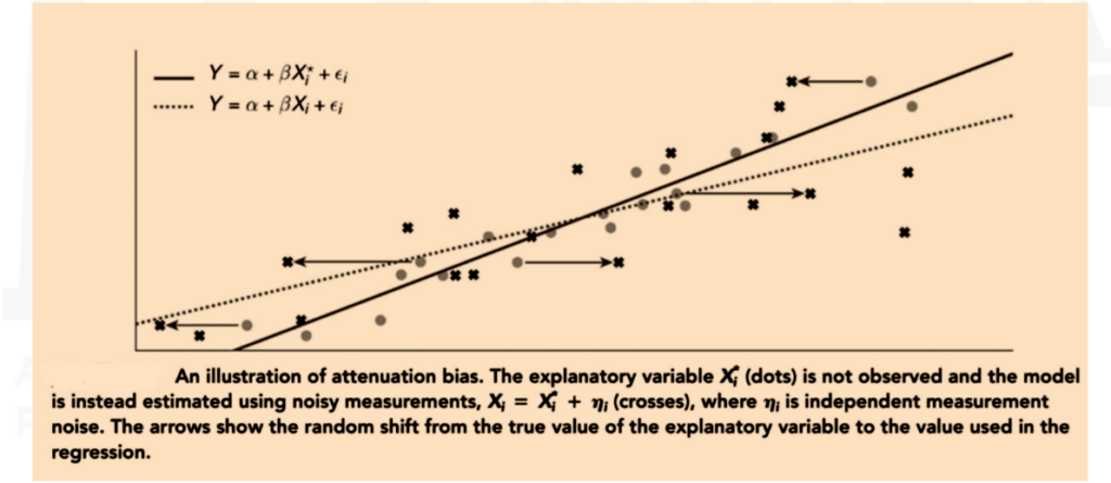
d)Attenuation bias
a) Sample selection bias or survivorship bias – Sample selection bias occurs when some observations are not recorded due to missing values of y_i. For example, when studying firm performance, the firms in operation are “winners” in the sense that they have performed well enough to continue to do business. Firms that are less successful are more likely to delist, and any model estimated using only the surviving firms is not representative of the behavior of all firms. Survivorship bias is commonly addressed using carefully constructed databases that report the final return for all firms, including those that delist.
b) Simultaneity bias – When X and Y are simultaneously determined, then modeling Y as a function of X is not meaningful because X is also a function of Y. The classic example of simultaneity bias is the relationship between quantities transacted and the transaction price. Changing the transaction price affects the quantity traded, which in turn affects the price.
c) Omitted variables – This occurs when the model excludes variables that are important determinants of Y. Omitting these creates coefficients that are biased and may indicate a relationship when there is, in fact, none.
d) Attenuation bias – When explanatory variables are measured with error, the estimated slopes are smaller in magnitude than the true slopes. This is because measurement error attenuates the relationship between Y and X, leading to inconsistent parameter estimates.
2) Data Are Realizations From i.i.d. Random Variables – Formally, it is assumed that the pairs (xi , yi) are iid draws from their joint distribution. This assumption allows xi and yi to be simultaneously generated.
3) Variance of X – The variance of X is strictly greater than 0. (i.e., σx2 > 0).
4) No correlation between error terms – The error terms should be uncorrelated across all observations, i.e.
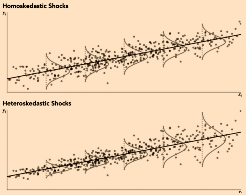
5) Constant Variance of Shocks – The variance of the shocks is finite and does not vary with Xi so that:
This assumption is known as homoskedasticity and requires that the variance of all shocks is the same.
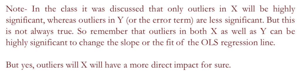
6) No Outliers – The probability of large outliers in X should be small. Outliers lead to large increases in the sum of squared errors, and parameters estimated using OLS in the presence of outliers may differ substantially from the true parameters. A single outlier in the error has the potential to substantially alter the fitted line. The simplest method to detect and address outliers is to visually examine data for extreme observations by plotting both the explanatory variables and the fitted residuals.


Properties of Ols Slope Estimator
- In practice, CLT is used as an approximation so that β ̂ is treated as a normal random variable that is centered at the true slope 𝛽:
- The variance of β ̂ increases with σ2 .
- On the other hand, the variance of β ̂ is decreasing in σX2.
- The effect of the sample size n is clear in this approximation: the variance of β ̂ decreases as the sample size increases
- The standard form of the estimator of the variance of β ̂ is
- The estimated standard error of β ̂ is hence, given by
The variance of the slope estimator depends on two moments: the variance of the shocks (i.e., σ2 ) and the variance of the explanatory variables (i.e., σX2).


properties of Ols Intercept Estimator
- The estimator for the variance of α ̂ can be constructed as
- The estimation error in α ̂ also depends on the variance of the residuals and the variance of X. In addition, it depends on μX2 (i.e., the squared mean of X). If X has mean 0 (i.e., μX = 0), then the asymptotic variance simplifies to σ2 and α ̂ simply estimates the mean of 𝑌.
where
the numerator uses a simplification derived from the identity
Inference and Hypothesis Testing
- When the assumptions in of OLS are satisfied, the estimators of α and β are normally distributed in large samples. Therefore, testing a hypothesis about a regression parameter is identical to testing a hypothesis about the mean of a random variable (or any other estimator that follows a CLT). Tests are implemented using a 𝑡-test, which measures the normalized difference between the estimated parameter and the value specified by the null hypothesis. When testing the null H0 : β = β0, the test statistic is
- The test is implemented by comparing the test statistic value to the critical values from a standard normal distribution. When the alternative is two-sided (e.g., H1 : β≠β0), then the null is rejected when:
- The test statistic can also be transformed into a p-value, which measures the probability of observing a test statistic as large as the one observed if the null is true. The p-value is computed by measuring the area in both tails that is beyond the test statistic. It is computed by first measuring the area in the right tail beyond the test statistic, 1-Φ(|T|), and then doubling this to account for both tails so that:
- The asymptotic distribution can also be used to construct confidence intervals using the quantiles of a standard normal distribution. A (1-c) confidence interval contains the set of null hypothesis values that are not rejected when using a significance level / test size of c. For example, the 90% confidence interval for β is
- It is common to report the 𝑡-statistic of the regression coefficient, which is the value of the test statistic for the specific null hypothesis that the parameter is 0.
- The asymptotic variance of the slope depends on the variance of the explanatory variable and the variance of the shocks. These two values can be estimated using only the elements of the covariance matrix between the dependent and the explanatory variables. It can be shown that:
- The variance of the innovations can be estimated using
- The mean annual excess returns of the mining sector (Y) and the market (X) are y ̅= 15.4% and x ̅=7.77%. The covariance matrix for the two annual returns is
|t| > Cs
where
Cs is the critical value from the normal distribution for a test with significance level (or size) s.
where
Φ(z) is the CDF of a standard normal.
where
ρ ̂XY is the sample correlation between the dependent and the explanatory variables.
Go to Syllabus
Courses Offered
Popular Courses
FRM Part 1
FRM Part 2

By : Micky Midha
9 Hrs of Videos
Available On Web, IOS & Android
Access Until You Pass
Lecture PDFs
Class Notes

By : Micky Midha
12 Hrs of Videos
Available On Web, IOS & Android
Access Until You Pass
Lecture PDFs
Class Notes

By : Micky Midha
257 Hrs Of Videos
Available On Web, IOS & Android
Access Until You Pass
Complete Study Material
Quizzes,Question Bank & Mock tests

By : Micky Midha
240 Hrs Of Videos
Available On Web, IOS & Android
Access Until You Pass
Complete Study Material
Quizzes,Question Bank & Mock tests

By : Shubham Swaraj
Lecture Videos
Available On Web, IOS & Android
Complete Study Material
Question Bank & Lecture PDFs
Doubt-Solving Forum