Introduction

• Forward prices and futures prices are related to the spot price of the underlying asset.
• Forward contracts are easier to analyze than futures contracts because there is no daily settlement only a single payment at maturity.
• It can be shown that the forward price and futures price of an asset are usually very close when the maturities of the two contracts are the same. This is convenient because it means that results obtained for forwards can be assumed to be true for futures.

Investment Assets Versus Consumption Assets

• An investment asset is an asset that is held solely for investment purposes by at least some traders. Stocks and bonds are clearly investment assets. Gold and silver are also examples of investment assets. It is not necessary that investment assets have to be held exclusively for investment. (Silver, for example, has a number of industrial uses.) However, they do have to satisfy the requirement that they are held by some traders solely for investment.
• A consumption asset is an asset that is held primarily for consumption. It is not normally held for investment. Examples of consumption assets are commodities such as copper, crude oil, corn, and pork bellies.
• Arbitrage arguments can be used to determine the forward and futures prices of an investment asset from its spot price and other observable market variables. This cannot be done for consumption assets.

Short Selling

• Short Selling, usually referred to as “shorting”, involves selling an asset that is not owned. It is something that is possible for some-but not all investment assets. It can be illustrated by considering a short sale of shares of a stock.
• If an investor wants to short sell a specific number of shares of company X, the broker will borrow the shares on the investor’s behalf from someone who owns them and sell them in the market in the usual way. At some later stage, the investor will close out the position by purchasing the same number of shares of company X in the market. These shares are then used to replace the borrowed shares so that the short position is closed out. If at any time while the contract is open the broker has to return the borrowed shares and there are no other shares that can be borrowed, the investor is forced to close out the position, even if not ready to do so. Often a fee is charged for lending the shares to the party doing the shorting.
• An investor with a short position must pay to the broker any income, such as dividends or interest, that would normally be received on the securities that have been shorted. The broker will transfer this income to the account of the client from whom the securities have been borrowed.

• For example, consider the position of an investor who shorts 500 shares in April when the price per share is $120. Suppose that a dividend of $1 per share is paid in May. The investor receives

500 × $120 = $60,000

in April when the short position is initiated.

The dividend in May leads to the investor paying

500× $1 = $500

Let’s assume further that the investor closes out the position by buying them back in July when the price per share is $100. So the investor also pays

500× $100 = $50,000

for shares when the position is closed out in July.

The net gain, therefore, is

$60,000-$500-$50,000=$9,500

when any fee for borrowing the shares is ignored.

• This table illustrates this example and shows that the cash flows from the short sale are the mirror image of the cash flows from purchasing the shares in April and selling them in July. The fee for borrowing the shares is not considered here.

Purchase of Shares
April – Purchase 500 shares @ $120	-$60,000
May – Receive dividend	+$500
July – Sell Shares @ 100	+$50,000
	Net profit= -$9,500
Short Sale of Shares
April: Borrow 500 shares and sell them @ $120	+$60,000
May – Pay dividend	-$500
July – Buy 500 shares @ $100 per share and Replace borrowed shares to close short position	-$50,000
	Net profit= +$9,500

• The investor is required to maintain a margin account with the broker. The margin account consists of cash or marketable securities deposited by the investor with the broker to guarantee that the investor will not walk away from the short position if the share price increases. It is similar to the margin account for futures contracts. An initial margin is required and if there are adverse movements (i.e., increases) in the price of the asset that is being shorted, additional margin may be required. If the additional margin is not provided, the short position is closed out. The margin account does not represent a cost to the investor. This is because interest is usually paid on the balance in margin accounts.
• From time to time regulations are changed on short selling. In 1938, the uptick rule was introduced. This allowed shares to be shorted only on an “uptick”-that is, when the most recent movement in the share price was an increase. The SEC abolished the uptick rule in July 2007, but introduced an “alternative uptick” rule in February 2010. Under this rule, when the price of a stock has decreased by more than 10% in one day, there are restrictions that the stock can be shorted only at a price that is higher than the best current bid price. Occasionally there are temporary bans on short selling. This happened in a number of countries in 2008.

Assumptions and Notation

• In this chapter, the following will be assumed for true-or at least approximately true-for a few key market participants such as large derivatives dealers, if not all participants:
  • The market participants are subject to no transaction costs when they trade.
  • The market participants are subject to the same tax rate on all net trading profits.
  • The market participants can borrow money at the same risk-free rate of interest as they can lend money.
  • The market participants take advantage of arbitrage opportunities as they occur.

• The following notation will be used throughout this chapter:
  • T – Time until delivery date in a forward or futures contract (in years)
  • 
    – Price of the asset underlying the forward or futures contract today
  • 
    – Forward or futures price today
  • r – Zero-coupon risk-free rate of interest per annum, expressed with continuous compounding, for an investment maturing at the delivery date(i.e., in T years).

Forward Price for an Investment Asset – An Example

• The easiest forward contract to value is one written on an investment asset that provides the holder with no income and for which there are no storage costs. Non dividend paying stocks and zero-coupon bonds are examples of such investment assets.
• Consider a long forward contract to purchase a non-dividend-paying stock in 3 months. Assume the current stock price is $40 and the 3-month risk-free interest rate is 5% per annum.
  • CASE I – Suppose first that the forward price is relatively high at $43. An arbitrageur can borrow $40 at the risk-free interest rate of 5% per annum, buy one share, and short a forward contract to sell one share in 3 months. At the end of the 3 months, the arbitrageur delivers the share and receives $43. The sum of money required to pay off the loan is

Hence the arbitrageur locks in a profit of

$43.00 – $40.50 = $2.50

at the end of the 3-month period.

• • CASE II – Suppose next that the forward price is relatively low at $39. An arbitrageur can short one share, invest the proceeds of the short sale at 5% per annum for 3 months, and take a long position in a 3-month forward contract. The proceeds of the short sale grow to

in 3 months.

At the end of the 3 months, the arbitrageur pays $39, takes delivery of the share under the terms of the forward contract, and uses it to close out the short position. Hence the arbitrageur locks in a profit of

$40.50 – $39.00 = $1.50

at the end of the 3-month period.

• The first arbitrage works when the forward price is greater than $40.50. The second arbitrage works when the forward price is less than $40.50. Hence it can be deduced that the no-arbitrage the forward price must be exactly $40.50.

Forward Price for an Investment Asset – An Example

• The two trading strategies we have considered are summarized in this table

CASE I – FORWARD PRICE=$43	CASE II – FORWARD PRICE=$39
Action now:	Action now:
Borrow $40 at 5% for 3 months Buy one unit of asset Enter into forward contract to sell asset in 3 months for $43	Short 1 unit of asset to realize $40 Invest $40 at 5% for 3 months Enter into a forward contract to buy asset in 3 months for $39
Action in 3 months:	Action in 3 months:
Sell asset for $43 Use $40.50 to repay loan with interest	Sell asset for $43 Use $40.50 to repay loan with interest
Profit realized = $2.50	Profit realized = $1.50

Forward Price for an Investment Asset – A Generalization

• The previous example can be generalized for a forward contract on an investment asset with price
  
  that provides no income. If T is the time to maturity, r is the risk-free rate,
  is the forward price, then the relationship between
  
  and
  
  is

• If
  , arbitrageurs can buy the asset and short forward contracts on the asset.
• If
  , they can short the asset and enter into long forward contracts on it.
• If short sales are not possible, investors who own the asset will find it profitable to sell the asset and enter into long forward contracts.
• In the previous example,
  
  = 40, r = 0.05 and T = 0.25, so

which is in agreement with our earlier calculations.

Forward Price for an Investment Asset – An Example

• Consider a 4-month forward contract to buy a zero-coupon bond that will mature 1 year from today. (This means that the bond will have 8 months to go when the forward contract matures.) The current price of the bond is $930. If the 4-month risk-free rate of interest (continuously compounded) is 6% per annum, then find the forward price.

Forward Price for an Investment Asset with Income

• Assets that provide a perfectly predictable cash income to the holder include stocks paying known dividends and coupon-bearing bonds. Consider a forward contract with 9-month maturity to purchase a coupon paying bond whose current price is $900, and a coupon payment of $40 is expected on the bond after 4 months. The 4-month and 9-month risk-free interest rates (continuously compounded) are, respectively, 3% and 4% per annum.
  • CASE I – Suppose first that the forward price is relatively high at $910. An arbitrageur can borrow $900 to buy the bond and enter into the forward contract to sell the bond for $910. The coupon payment has a present value of

Of the $900, $39.60 is therefore borrowed at 3% per annum for 4 months so that it can be repaid with the coupon payment. The remaining $860.40 is borrowed at 4% per annum for 9 months. The amount owing at the end of the 9-month period is

A sum of $910 is received for the bond under the terms of the forward contract. The arbitrageur therefore makes a net profit of

910.00 – 886.60 = $23.40

• • CASE II – Suppose next that the forward price is relatively low at $870. An investor can short the bond and enter into the forward contract to buy the bond for $870. Of the $900 realized from shorting the bond, $39.60 is invested for 4 months at 3% per annum so that it grows into an amount

after four months, which is sufficient to pay the coupon on the bond. The remaining $860.40 is invested for 9 months at 4% per annum and grows to

Under the terms of the forward contract, $870 is paid to buy the bond and the short position is closed out. The investor therefore gains

886.60-870=$16.60

• The first strategy produces a profit when the forward price is greater than $886.60, whereas the second strategy produces a profit when the forward price is less than $886.60. It follows that if there are no arbitrage opportunities then the forward price must be $886.60.

Forward Price for an Investment Asset with Known Income

The two strategies are summarized in this table

CASE I – FORWARD PRICE=$910	CASE II – FORWARD PRICE=$870
Action now	Action now
Borrow $900: $39.60 for 4 months and $860.40 for 9 months Buy one unit of asset Enter into forward contract to sell asset in 9 months for $910	Short 1 unit of asset to realize $40 Invest $39.60 at 3% for 4 months and $860.40 at 4% for 9 months Enter into a forward contract to buy asset in 9 months for $870
Action in 4months:	Action in 4months:
Receive $40 of income on asset Use $40 to repay first loan with interest	Receive $40 of income on asset Use $40 to repay first loan with interest
Action in 9 months	Action in 9 months
Receive $40 of income on asset Use $40 to repay first loan with interest	Receive $40 of income on asset Use $40 to repay first loan with interest
Profit realized = $23.40	Profit realized = $16.60

• This previous example can be generalized to

where

I is present value of income provided by the investment asset during the life of a forward contract

• • If
    , an arbitrageur can lock in a profit by buying the asset and shorting a forward contract on the asset
  • If
    , an arbitrageur can lock in a profit by shorting the asset and taking a long position in a forward contract.
  • If short sales are not possible, investors who own the asset will find it profitable to sell the asset and enter into long forward contracts.
• In our previous example,
  
  = 900.00,
  

So that

which is in agreement with our earlier calculation.

• Example

Consider a 10-month forward contract on a stock when the stock price is $50. We assume that the risk-free rate of interest (continuously compounded) is 8% per annum for all maturities and also that dividends of $0.75 per share are expected after 3 months, 6 months, and 9 months.

• If the asset underlying a forward contract provides a known yield rather than a known cash, then it can be shown that

• Example –

Consider a 6-month forward contract on an asset with

= 25, that is expected to provide income equal to 2% of the asset price once during a 6-month period. The risk-free rate of interest (with continuous compounding) is 10% per annum. The asset price is $25.

Valuing Forward Contracts

• The value of a forward contract at the time it is first entered into is close to zero. At a later stage, it may prove to have a positive or negative value. Following notations will be used
  • K is the delivery price for a contract that was negotiated some time ago,
  • The delivery date is T years from today,
  • r is the T-year risk-free interest rate.
  • The variable
    
    is the forward price that would be applicable if the contract was negotiated today.
  • In addition, f is defined to be the value of forward contract today.
• It is important to be clear about the meaning of the variables
  , K and f. At the beginning of the life of the forward contract,
  • The delivery price, K, is set equal to the forward price at that time
  • The value of the contract, f, is 0.

As time passes, K stays the same (because it is part of the definition of the contract), but the forward price changes and the value of the contract becomes either positive or negative.

• A general result, applicable to all long forward contracts (both those on investment assets and those on consumption assets), is

And the value of a (short) forward contract to sell the asset for Kat time Tis

• Example

A long forward contract on a non-dividend-paying stock was entered into some time ago. It currently has 6 months to maturity. The risk-free rate of interest (with continuous compounding) is 10% per annum, the stock price is $25, and the delivery price is $24.

Valuing Forward Contracts for Assets with Income/Yield

• The value of a long forward contract on an investment asset that provides a known income with present value I is

• The value of a long forward contract on an investment asset that provides a known yield at rate q:

• When a futures price changes, the gain or loss on a futures contract is calculated as the change in the futures price multiplied by the size of the position. This gain is realized almost immediately because futures contracts are settled daily. when a forward price changes, the gain or loss is the present value of the change in the forward price multiplied by the size of the position.

Forward Prices Versus Futures Prices

• For no arbitrage, when the short-term risk-free interest rate is constant, the forward price for a contract with a certain delivery date is in theory the same as the futures price for a contract with that delivery date.
• When interest rates vary unpredictably (as they do in the real world), forward and futures prices are in theory no longer the same.
  • Case I – The price of the underlying asset, S, is strongly positively correlated with interest rates. When S increases, an investor who holds a long futures position makes an immediate gain because of the daily settlement procedure. The positive correlation indicates that it is likely that interest rates have also increased, thereby increasing the rate at which the gain can be invested. Similarly, when S decreases, the investor will incur an immediate loss and it is likely that interest rates have just decreased, thereby reducing the rate at which the loss has to be financed. So gains are amplified and losses are reduced. An investor holding a forward contract rather than a futures contract is not affected in this way by interest rate movements. It follows that a long futures contract will be slightly more attractive than a similar long forward contract. Hence, when S is strongly positively correlated with interest rates, futures prices will tend to be slightly higher than forward prices.

Are Forward Prices and Futures Prices Equal?

• Case II – The price of the underlying asset, S, is strongly negatively correlated with interest rates. When S increases, an investor who holds a long futures position makes an immediate gain because of the daily settlement procedure. The negative correlation indicates that it is likely that interest rates have decreased, thereby decreasing the rate at which the gain can be invested. Similarly, when S decreases, the investor will incur an immediate loss and it is likely that interest rates have just increased, thereby increasing the rate at which the loss has to be financed. So gains are reduced and losses are amplified. An investor holding a forward contract rather than a futures contract is not affected in this way by interest rate movements. It follows that a long futures contract will be slightly less attractive than a similar long forward contract. Hence, when S is strongly negatively correlated with interest rates, futures prices will tend to be slightly lower than forward prices.

Futures Prices of Stock Indices

• A stock index can usually be regarded as the price of an investment asset that pays dividends. The investment asset is the portfolio of stocks underlying the index, and the dividends paid by the investment asset are the dividends that would be received by the holder of this portfolio. If q is the dividend yield rate (with continuous compounding), then the futures price,
  , is

In practice, the dividend yield on the portfolio underlying an index varies week by week throughout the year. The chosen value of q should represent the average annualized dividend yield during the life of the contract.

• Example – Consider a 3-month futures contract on an index. Suppose that the stocks underlying the index provide a dividend yield of 1% per annum (continuously compounded), that the current value of the index is 1,300, and that the continuously compounded risk-free interest rate is 5% per annum.

Index Arbitrage

• If
  , profits can be made by buying the stocks underlying the index at the spot price (i.e., for immediate delivery) and shorting futures contracts. In this case, index arbitrage it might be done by a bank or a corporation holding short-term money market investments.
• If
  , profits can be made by doing the reverse-that is, shorting or selling the stocks underlying the index and taking a long position in futures contracts. In this case, index arbitrage is often done by a pension fund that owns an indexed portfolio of stocks.
• For indices involving many stocks, index arbitrage is sometimes accomplished by trading a relatively small representative sample of stocks whose movements closely mirror those of the index. Usually index arbitrage is implemented through program trading. This involves using a computer system to generate the trades.

Forward and Futures Contracts on Currencies

• For the sake of definiteness it will be assumed that the domestic currency is the U.S. dollar (i.e., the perspective of a U.S. investor will be taken). The underlying asset is one unit of the foreign currency.
  • The variable
    
    is defined as the current spot price in U.S. dollars of one unit of the foreign currency
  • 
    as the forward or futures price in U.S. dollars of one unit of the foreign currency.
• It is not necessary that the above convention corresponds to the way spot and forward exchange rates are quoted. For major exchange rates other than the British pound, euro, Australian dollar, and New Zealand dollar, a spot or forward exchange rate is normally quoted as the number of units of the currency that are equivalent to one U.S. dollar.
• A foreign currency has the property that the holder of the currency can earn interest at the risk-free interest rate prevailing in the foreign country. For example, the holder can invest the currency in a foreign-denominated bond.
  • 
    , is defined to be as the value of the foreign risk-free interest rate when money is invested for time T.
  • r is the domestic risk-free rate when money is invested for this period of time.

• The relationship between
  
  and
  
  is

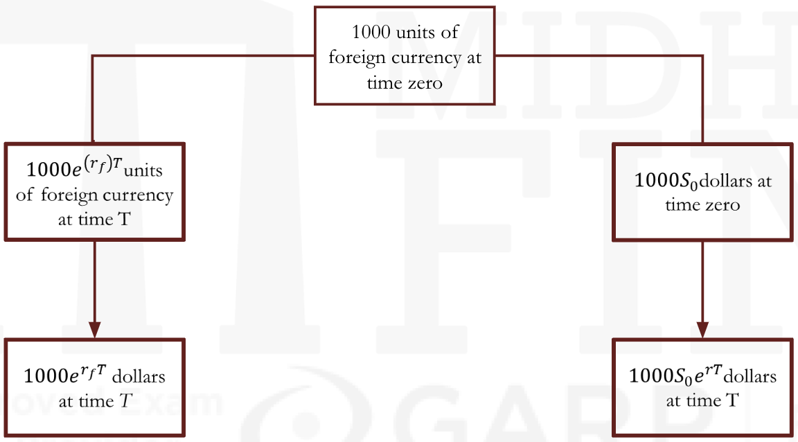
• This is the well-known interest rate parity relationship from international finance. For example, suppose that an individual starts with 1,000 units of the foreign currency. There are two ways it can be converted to dollars at time T. One is by investing it for T years at
  
  and entering into a forward contract to sell the proceeds for dollars at time T. This generates
  
  dollars. The other is by exchanging the foreign currency for dollars in the spot market and investing the proceeds for T years at rater. This generates
  
  dollars.

In the absence of arbitrage opportunities, the two strategies must give the same result. Hence,

=

So that

• The previous example is depicted in this figure

• Example 1 –

The forward rate of a 3-month EUR/USD foreign exchange contract is 1.1565 USD per EUR. USD LIBOR is 4% and EUR LIBOR is 2%. Find the spot USD per EUR exchange rate.

Currency Forward Arbitrage – Example

• Given the following:

Current spot CHF/USD rate – 1.3680 (CHF 1.3680 = USD 1)

3-month USD interest rates: 1.05% ; 3-month Swiss interest rates: 0.35%

A currency trader notices that the 3-month forward price is USD/CHF 0.7350.

Is arbitrage possible. If yes, what should be the strategy ?

Futures on Commodities

• Let's consider futures contracts on commodities, and start with commodities that are investment assets such as gold and silver. In the absence of storage costs and income, the forward price of a commodity that is an investment asset is given by

• Storage costs can be treated as negative income. If U is the present value of all the storage costs, net of income, during the life of a forward contract, it follows from equation (8.2) that

• If the storage costs (net of income) incurred at any time are proportional to the price of the commodity, they can be treated as negative yield. In this case,

where u denotes the storage costs per annum as a proportion of the spot price net of any yield earned on the asset.

• If
  , then to take advantage of this opportunity, an arbitrageur can implement the following strategy:
  • Borrow an amount
    
    at the risk-free rate and use it to purchase one unit of the commodity and to pay storage costs.
  • Short a futures contract on one unit of the commodity.

If the futures contract is treated as a forward contract, so that there is no daily settlement, this strategy leads to a profit of

at time T.

• If
  , then to take advantage of this opportunity, an arbitrageur can implement the following strategy:
  • Sell the commodity, save the storage costs, and invest the proceeds at the risk-free interest rate.
  • Take a long position in a futures contract.

If the futures contract is treated as a forward contract, so that there is no daily settlement, this strategy leads to a profit of

at time T.

Futures on Commodities – Example

• Consider a 1-year futures contract on an investment asset that provides no income. It costs $2 per unit to store the asset, with the payment being made at the end of the year. Assume that the spot price is $450 per unit and the risk-free rate is 7% per annum for all maturities.
• If the actual futures price is greater than ___________, an arbitrageur can buy the asset and short 1-year futures contracts to lock in a profit. If the actual futures price is less than ____________, an investor who already owns the asset can improve the return by selling the asset and buying futures contracts.

Futures on Commodities

• The previous arbitrage argument cannot be used for a commodity that is a consumption asset rather than an investment asset. Individuals and companies who own a consumption commodity usually plan to use it in some way. They are reluctant to sell the commodity in the spot market and buy forward or futures contracts, because forward and futures contracts cannot be used in a manufacturing process or consumed in some other way. For example, crude oil in inventory can be an input to the refining process, whereas a futures contract cannot be used for this purpose. In general, ownership of the physical asset enables a manufacturer to keep a production process running and perhaps profit from temporary local shortages. A futures contract does not do the same.
• So it can be asserted that for a consumption commodity

If storage costs are expressed as a proportion u of the spot price, the equivalent result is

Convenience Yields

• The benefits from holding the physical asset are sometimes referred to as the convenience yield provided by the commodity. If the dollar amount of storage costs is known and has a present value U, then the convenience yield y is defined such that

If the storage costs per unit are a constant proportion, u, of the spot price, then

• The convenience yield simply measures the extent to which the left-hand side is less than the right-hand side in the inequality
  . For investment assets the convenience yield must be zero; otherwise, there are arbitrage opportunities. The convenience yield reflects the market's expectations concerning the future availability of the commodity. The greater the possibility that shortages will occur, the higher the convenience yield. If users of the commodity have high inventories, there is very little chance of shortages in the near future and the convenience yield tends to be low. If inventories are low, shortages are more likely and the convenience yield is usually higher.

The Cost of Carry

• The relationship between futures prices and spot prices can be summarized in terms of the cost of carry. This measures the storage cost plus the interest that is paid to finance the asset less the income earned on the asset.
  • For a non-dividend-paying stock, the cost of carry is r, because there are no storage costs and no income is earned
  • For a stock index, it is (r – q), because income is earned at rate q on the asset.
  • For a currency, it is
    .
  • For a commodity that provides income at rate q and requires storage costs at rate u, it is (r – q + u);
• If the cost of carry is defined as c, then
  • For an investment asset, the futures price is
    
  • For a consumption asset, it is
    
    where y is convenience yield

Delivery Options

• Whereas a forward contract normally specifies that delivery is to take place on a particular day, a futures contract often allows the party with the short position to choose to deliver at any time during a certain period. (Typically the party has to give a few days' notice of its intention to deliver.) The choice introduces a complication into the determination of futures prices with regards to the maturity of the futures contract.
• If the futures price is an increasing function of the time to maturity, then c > y, so that the benefits from holding the asset (including convenience yield and net of storage costs) are less than the risk-free rate. It is usually optimal in such a case for the party with the short position to deliver as early as possible, because the interest earned on the cash received outweighs the benefits of holding the asset. As a rule, futures prices in these circumstances should be calculated on the basis that delivery will take place at the beginning of the delivery period.
• If futures prices are decreasing as time to maturity increases (c < y), the reverse is true. It is then usually optimal for the party with the short position to deliver as late as possible, and futures prices should, as a rule, be calculated on this assumption.

Futures Prices and Expected Future Spot Prices

• The expected spot price of an asset at a certain future time is the market's average opinion about what the spot price of an asset will be at that future time. It is already known that the futures price converges to the spot price at maturity. If the expected spot price is less than the current futures price, the market must be expecting the futures price to decline, so that traders with short positions gain and traders with long positions lose. If the expected spot price is greater than the current futures price, the market must be expecting the futures price to increase, so that traders with long positions gain while those with short positions lose.
• Economists John Maynard Keynes and John Hicks argued that, if hedgers tend to hold short positions and speculators tend to hold long positions, the futures price of an asset will be below the expected spot price. This is because speculators require compensation for the risks they are bearing. They will trade only if they can expect to make money on average. Hedgers will lose money on average, but they are likely to be prepared to accept this because the futures contract reduces their risks. If hedgers tend to hold long positions while speculators hold short positions, Keynes and Hicks argued that the futures price will be above the expected spot price for a similar reason.

Risk and Return

• In general, the higher the risk of an investment, the higher the expected return demanded by an investor. The capital asset pricing model, states that there are two types of risk in the economy: systematic and nonsystematic. Nonsystematic risk should not be important to an investor. It can be almost completely eliminated by holding a well-diversified portfolio. An investor should not therefore require a higher expected return for bearing nonsystematic risk. Systematic risk, in contrast, cannot be diversified away. It arises from a correlation between returns from the investment and returns from the whole stock market. An investor generally requires a higher expected return than the risk-free interest rate for bearing positive amounts of systematic risk. Also, an investor is prepared to accept a lower expected return than the risk-free interest rate when the systematic risk in an investment is negative.
• It can be shown that the futures price is an unbiased estimate of the expected future spot price when the return from the underlying asset is uncorrelated with the stock market i.e.

where

is the futures price today,

is the price of the asset at time T, and

E denotes expected value.

The Risk in a Futures Position

• If the return from the asset is positively correlated with the stock market, then
  . This shows that, when the asset underlying the futures contract has positive systematic risk, then the futures price to understate the expected future spot price. An example of an asset that has positive systematic risk is a stock index. The expected return of investors on the stocks underlying an index is generally more than the risk-free rate, r. The dividends provide a return of q. The expected increase in the index must therefore be more than r-q.
• If the return from the asset is negatively correlated with the stock market, then
  . This shows that, when the asset underlying the futures contract has negative systematic risk, we should expect the futures price to overstate the expected future spot price.
• If k is the expected return from the asset, r is the risk-free rate,
  
  is the futures price and
  is the expected future spot price, then the relationship between Futures Price and Expected Future Spot Price is summarized as follows

Underlying Asset	Relationship of k and r	Relationship and
No systematic risk	k = r
Positive systematic risk	k > r
Negative systematic risk	k < r

Normal Backwardation and Contango

• Normal Backwardation and Normal Contango
  • When the futures price is below the expected future spot price, the situation is known as normal backwardation.
  • When the futures price is above the expected future spot price, the situation is known as normal contango.
• Backwardation and Contango
  • When futures price is below the current spot price, rather than the expected future spot price, the situation is known as
    backwardation.
  • When futures price is above the current spot price, rather than the expected future spot price, the situation is known as contango.