Introduction

•This chapter presents a framework for understanding the shape of the term structure. In  particular, it is shown how spot or forward rates are determined by expectations of future  short-term rates, the volatility of short-term rates, and an interest rate risk premium.

•For equilibrium models, an understanding of the relationships between the model assumptions  and the shape of  the term structure is important in order to make reasonable assumptions in  the first place. For arbitrage-free models, an understanding of these relationships reveals the  assumptions implied by the market through the observed term structure.

•The more modest goal of this chapter is to connect the dynamics of the short-term rate of  interest and the risk premium with the shape of the term structure. While this goal does fall  short of answers that an economist might provide with respect to factors such as the marginal  productivity of capital, the propensity to save, expected inflation, etc., it is more ambitious than  the derivation of arbitrage restrictions on bond and derivative prices given underlying bond  prices.

Expectations

•The word expectations implies uncertainty. Investors might expect the one-year rate to be 10%,  but know there is a good chance it will turn out to be 8% or 12%. Expectations play an  important role in determining the shape of  the yield curve which can be flat, upward-sloping,  and downward-sloping.

•EXAMPLE – Role of interest rate forecasts in determining the shape of the term structure

Let’s start by assuming that there is no  uncertainty so that the statement that investors expect or forecast a rate of 10% means that investors assume that the rate will be 10%. The one-year  interest rate is currently 10% and all investors forecast that the one-year interest rate next year  and the year after will also be 10%. In that case, investors will discount cash flows using  forward rates of 10%. In particular, the price of  𝑜𝑛𝑒-, 𝑡𝑤𝑜- and 𝑡ℎ𝑟𝑒𝑒-year zero-coupon  bonds per dollar face value (using annual compounding) will be

The term structure of spot rates in this example is flat at 10%. Very simply, investors  are willing to lock in 10% for two or three years because they assume that the one-year rate will always be 10%.

•Now let’s assume that the one-year rate is still 10%, but that all investors forecast the one-year  rate next year to be 12% and the one-year rate in two years to be 14%. Using the forward rate  concept from FRM Part 1, the two-year spot rate, 𝑟̂ 2 , is such that

Solving, 𝑟̂ 2 =10.995% . Similarly, the three-year spot rate, 𝑟̂ 3 , is such that

Solving, 𝑟̂ 3  = 11.998%. Hence, the evolution of  the one-year rate from 10% to 12% to  14% generates an upward sloping term structure of spot rates: 10%,  10.995%,  and  11.988%.

In this case, investors require rates above 10% when locking up their money for two or three  years because they assume one-year rates will be higher than 10%. No investor, for example,  would buy a two-year zero at a yield of 10% when it is possible to buy a one-year zero at 10% and, when it matures, buy another one-year zero at 12%.

•  Finally, assume that the one-year rate is 10%, but that investors forecast that it will fall to 8%  in one year and to 6% in two years. In that case, it is easy to show that the term structure of  spot rates will be downward-sloping. In particular,

𝑟̂(1) = 10% , 𝑟̂ 2  = 8.995%, and 𝑟̂(3) = 7.988%.

•These simple examples reveal that expectations can cause the term structure to take on any of a  myriad of shapes.

1. Over short horizons, the financial community can have very specific views about future  short-term rates.

2. Over longer horizons, however, expectations cannot be so granular. It would be difficult, for

example, to defend the position that the expectation for the one-year rate 29  years from  now is substantially different from the expectation of the one-year rate 30 years from now.  On the other hand, an argument can be made that the long-run expectation of the short-  term rate is 5%: 3% due to long-run real rate of interest and 2% due to long-run inflation.

•Hence, forecasts can be very useful in describing the shape and level of the term  structure over short-term horizons and the level of rates at very long horizons.

Volatility And Convexity

•This section drops the assumption that investors believe that their forecasts will be realized  and assumes instead that investors understand the volatility around their expectations. To  isolate the implications of  volatility on the shape of  the term structure, this section assumes  that investors are risk-neutral so that they price securities by expected discounted value. The  next section drops this assumption.

•Assume that the following tree gives the true process for the one-year rate:

•The expected interest rate on date 1 is

0.5 × 8% + 0.5 × 12% = 10%

•The expected rate on date 2 is

0.25 × 14% + 0.5 × 10% + 0.25 × 6% = 10%

•In the previous section, with no volatility around  expectations, flat expectations of 10% imply a flat term  structure of spot rates. That is not the case in the presence  of volatility.

•The price of a one-year zero is, by definition, 1/1.10 = 0.909091, implying a one-year spot rate of 10%.

•Under the assumption of  risk-neutrality, the price of  a two-year zero may be calculated by  discounting the terminal cash flow using the preceding interest rate tree:

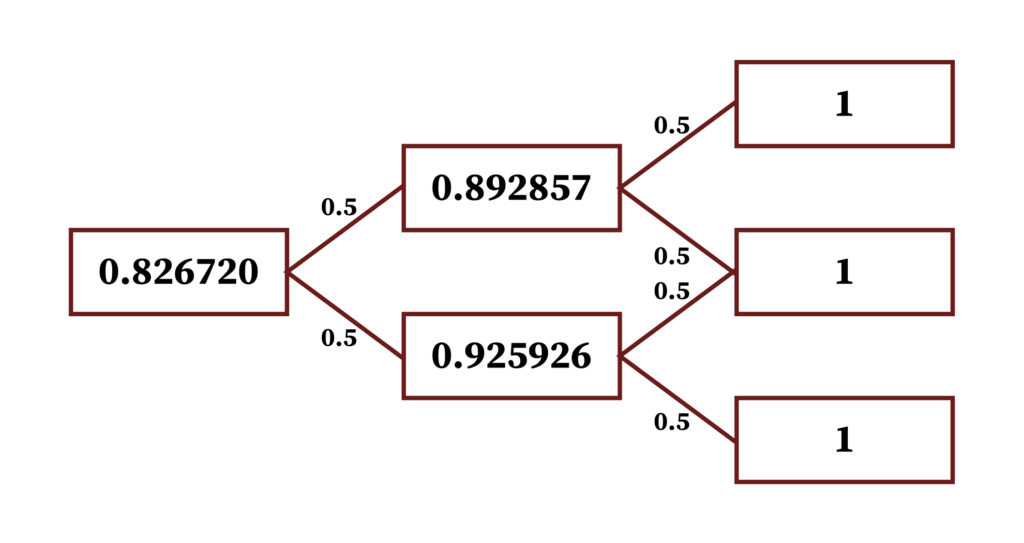
Hence, the two-year spot rate is such that 0.82672 = 1 / 1 + r^2 which gives r^(2) = 9.982%.

•The tree presented at the start of this section may also be used to price a three-year zero. The resulting price tree is

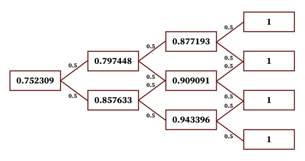
•The three-year spot rate, such that 0.752309 = 1 / (1 + r^(3))^3, which gives r^3 = 9.9525.Therefore, the value of convexity in this spot rate is 10% — 9.952% or 4.8 basis points,  whereas the value of convexity in the two-year spot rate was only 1.8 basis points.

•It is generally true that, all else equal, the value of convexity increases with maturity. Securities  with greater convexity perform better when yields change a lot and perform worse when yields  do not change by much. Convexity does, in fact, lower bond yields.

•Furthermore, the value of convexity increases with volatility. In the tree introduced at the start  of the section, the standard deviation of rates is 200 basis points a year . Now consider a tree  with a standard deviation of 400 basis points. The expected one-year rate in one year and in two years is still 10%.  Spot rates and convexity values for this case may be  derived along the same lines as before.

•This figure graphs three term  structures of spot rates: one with no  volatility around the expectation of  10%; one with a volatility of 200  basis points a year (the tree of  the  first example); and one with a  volatility of 400 basis points per year  (the tree preceding this paragraph).  Note that the value of convexity,  measured by the  distance between  the rates assuming no volatility and  the rates assuming volatility, increases  with volatility.

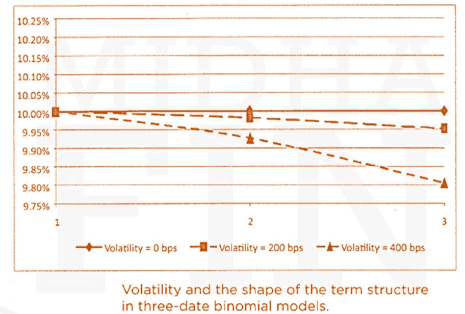
•This figure also illustrates that the value of convexity increases with maturity.

•For very short terms and realistic levels of volatility, the value of convexity is quite small.

Volatility and Convexity – Jensen’s Inequality

•Even though the one-year rate is 10% and the expected one-year rate in one year is 10%, the two-  year spot rate is 9.982%. The 1.8-basis point difference between the spot rate that would obtain in  the absence of uncertainty, 10%, and the spot rate in the presence of volatility, 9.982%, is the effect  of convexity on that spot rate. This convexity effect arises from the mathematical fact, a special case  of Jensen’s Inequality, that

•In our example, it can be shown the one-year spot rate is less than 10%. The spot rate one year from  now may be 12% or 8%. So according to Jensen’s inequality

Dividing both sides by 1.10 gives :-

The left-hand side of this inequality is the price of the two-year zero-coupon bond today. Hence, the  price of the two-year zero is greater than the result of discounting the terminal cash flow by 10%  over the first period and by the expected rate of 10% over the second period. It follows immediately that the yield of the two-year zero, or the two-year spot rate, is less than 10%.

Convexity-graphical Illustration of Jensen’s Inequality

•The  previous  figure  graphically  illustrates  the  inequality.  There  are  two  possible  values  of  𝑟 and, consequently, of the function  ¹  , in the figure shown as points A and D. The height or vertical-axis coordinate of  point B is the average of  these two function values. Under the assumption that the two possible values of 𝑟 occur with equal probability, this average can be thought of as 𝐸[1/1+r] . And under the same assumption, the horizontal-axis coordinates of the points Band C can be thought of as E[r] so that the height of point C can be thought of as 1 / 1 + E(r).

•Clearly, the height of B is greater than that of C, or

To summarize, Jensen’s inequality is true because the pricing function of  a zero-coupon bond, 1/ 1+r, ,is convex rather than concave.

Risk Premium

•To illustrate the effect of risk premium on the term structure, consider again the second interest  rate tree presented in the preceding section, with a volatility of 400 basis points per year. Risk-  neutral investors would price a two-year zero by the following calculation:

The return will, in fact, be either 6% or 14%. While these two returns do average to 10%, an  investor could, instead, buy a one year zero with a certain return of 10%. Presented with this  choice, any risk-averse investor would prefer an investment with a certain return of 10% to an  investment with a risky return that averages 10% . In other words, investors require  compensation for bearing interest rate risk. So risk-averse investors demand a return higher than  10% for the two-year zero over the next year. Future cash flows could be discounted at rates  higher than the possible rates of 14% and 6%. For example, adding 20 basis points to each of  these rates is equivalent to assuming that investors demand an extra 20  basis points for each  year of duration risk, the price of the two-year zero would be computed as follows:

•The price computed by risk-averse investors is below the risk-neutral price. In one year, if the interest rate is 14%, then the price of a one-year zero will 1/1.14 or 0.877193. If the rate is 6%, then the price will be 1 /1.06 or 0.943396.Therefore, the expected return of  the two-year zero priced at 0.826035 is

As the one-year zero has a certain return of 10%, the risk-averse investors in this example  demand 20 basis points in expected return to compensate them for the one year of duration  risk inherent in the two year zero.

Risk Premium and Convexity

•Continuing with the assumption of 400-basis-  point volatility, this figure graphs the term  structure of spot rates for three cases: no risk  premium, a risk premium of  20  basis points  per year of duration risk, and a risk premium of  40 basis points. In the case of no risk premium,  the term structure of spot rates is downward-  sloping due to convexity. A risk premium of 20  basis points pushes up spot rates while  convexity pulls them down. In the short end,  the risk premium effect dominates and the term  structure is mildly upward-sloping.

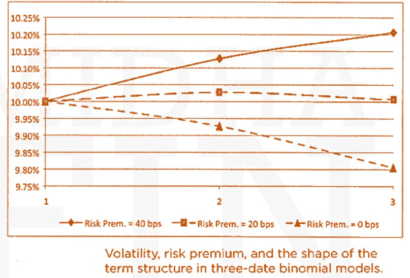
•In the long end, the convexity effect dominates and the term structure is mildly downward-  sloping.. Finally, a risk premium as large as 40 basis points dominates the convexity effect and  the term structure of spot rates is upward-sloping. The convexity effect is still evident, however,  from the fact that the curve increases more rapidly from one to two years than from two to three years.

Sources of Risk Premium

•Asset pricing theory (e.g., the Capital Asset Pricing Model, or CAPM) teaches that assets whose  returns are positively correlated with aggregate wealth or consumption will earn a risk premium.  Consider, for example, a traded stock index. That asset will almost certainly do well if the  economy is doing well and poorly if the economy is doing poorly. But investors, as a group,  already have a lot of exposure to the economy. To entice them to hold a little more of  the  economy in the form of a traded stock index requires the payment of a risk premium; i.e., the  index must offer an expected return greater than the risk-free rate of return. On the other hand,  say that there exists an asset that is negatively correlated with the economy. Holdings in that asset  allow investors to reduce their exposure to the economy. As a result, investors would accept an  expected return on that asset below the risk -free rate of  return. That asset, in other words,  would have a negative risk premium.

•This section assumes that bonds with interest rate risk earn a risk premium. In terms of asset  pricing theory, this is equivalent to assuming that bond returns are positively correlated with the  economy or, equivalently, that falling interest rates are associated with good times. One argument supporting this assumption is that interest rates fall when inflation and  expected inflation fall and that low inflation is correlated with good times.

•The concept of a risk premium in fixed income markets has probably gained favor more for its  empirical usefulness than for its theoretical solidity. On average, over the past 75 years, the term  structure of  interest rates has sloped upward.8 While the market may from time to time expect  that interest rates will rise, it is hard to believe that the market expects interest rates to rise on  average. Therefore, expectations cannot explain a term structure of interest rates that, on  average, slopes upward. Convexity, of course, leads to a downward-sloping term  structure.  Hence, of the three effects described in this chapter, only a positive risk premium can explain a  term structure that, on average, slopes upward.

•An uncomfortable fact, however, is that over earlier time periods the term structure has, on  average, been flat. Whether this means that an interest rate risk premium is a relatively recent  phenomenon that is here to stay or that the experience of persistently upward-sloping curves is  only partially due to a risk premium is a question beyond the scope of this book. In short, the  theoretical and empirical questions with respect to the existence of an interest rate risk premium  have not been settled.