Introduction

•This chapter uses a very simple setting to show how to price interest rate contingent claims   relative to a set of underlying securities by arbitrage arguments. Unlike the arbitrage pricing of   securities with fixed cash flows, the techniques of this chapter require strong assumptions about   how interest rates evolve in the future. This chapter also introduces option-adjusted spread (OAS) as the most popular measure of deviations of market prices from those predicted by models.

Rate and Price Trees

•Let’s assume that the six-month and one-year spot rates are 5% and  5.15%  respectively,  and  six months  from  now  the  six-month  rate  will  be  either  4.50%  or  5.50%  with  equal probability. This very strong assumption is depicted by means of a binomial tree. The six-month rate is 5% today, which will be called date 0. On the next date six months from now, which will be called date 1, there are two possible outcomes or states of the world. The 5.50% state will be called the up-state while the 4.50% state will be called the down-state.

•Given the current term structure of spot rates (i.e., the current   six-month and one-year rates), trees for the prices of six-month   and one-year zero-coupon bonds may be computed. The price   tree for $1,000 face value of the six month zero is hence

On date 0 of the preceding tree the security is a six-month zero, while on date 1 the security is a maturing zero.

•The  three  date  2  prices  of  $1,000 are,  of  course,  the   maturity values of the one-year zero. The two date 1 prices   come  from  discounting  this  certain  $1,000 at  the  then   prevailing six-month rate. Hence, the date 1 up-state price is

•And the date 1 down-state price is

•Finally, the date 0 price is computed using the given date 0 one-year rate of 5.5%:

•The probabilities of  moving up or down the tree may be used to compute the average or expected values. As of date 0, the expected value of the one-year zero’s price on date 1 is

Discounting this expected value to date 0 at the six-month rate (which is 5%) gives an expected discounted value of

•The one-year zero’s expected discounted value of $951.82 does not equal its given market price   of $950.42. These two numbers need not be equal because investors do not price securities by   expected discounted value. Over the next six months the one-year zero is a risky security, worth $973.24 half of the time and $978 the other half of the time for an average or expected value of $975.62. If investors do not like this price uncertainty, they would prefer a security worth $975.62 on date 1 with certainty. More specifically, a security worth $975.62 with certainty after six months would sell for $951.82 as of date 0. By contrast, investors penalize the risky one-year zero-coupon bond with an average price of $975.62 after six months by pricing it at $950.42 instead of $951.82.

Arbitrage Pricing of Derivatives

•Let’s  consider  a  call  option,  maturing  in  six  months,  to   purchase $1,000 face value of a then six-month zero at $975.   If  on date 1 the six-month rate is 5.50% and a six-month   zero sells for $973.23, the right to buy that zero at $975 is   worthless. But, if the six-month rate turns out to be 4.50%   and the price of a six-month zero is $978, then the right to   buy the zero at $975 is worth $978 — $975 = $3.

•A security is priced by arbitrage by finding and pricing its replicating portfolio. To price the option   by arbitrage, construct a portfolio on date 0 of underlying securities, namely six-month and one-   year zero-coupon bonds, that will be worth $0 in the up-state on date 1 and $3 in the down-state.   To solve this problem, let 𝐹^0.5and 𝐹¹ be the face values of six-month and one-year zeros in the   replicating portfolio, respectively. Then, these values must satisfy the following two equations:

1. 𝐹^0.5 + .97324𝐹¹ = $0 The left-hand side of  this equation is the value of  the replicating portfolio in the up-state, which must equal $0 (value of the option in the up-state).

2. 𝐹^0.5 + .97800𝐹¹ = $3 The left-hand side of this equation is the value of the replicating portfolio in the down-state, which must equal $3, (value of the option in the down-state).

•Solving the previous two equations gives

𝐹^0.5 = —$613.3866 and𝐹¹ = $630.2521

In words, on date 0 the replicating portfolio for the option can be created by buying about

$630.25 face value of one-year zeros and simultaneously shorting about $613.39 face amount of six-month zeros. This portfolio’s price is known and is equal to

—0.97561𝐹^0.5 + 0.95042𝐹¹ = —0.97561 × $613.3866 + 0.95042 × $630.2521 = $0.58

Since this is the case, the law of one price requires that the price of the option equal the price of the replicating portfolio.

Therefore, the price of the option must be $0.58 .

•The option cannot be priced by expected discounted value. Under that method, the option price would appear to be

The true option price is less than this value because investors dislike the risk of the call option and, as a result, will not pay as much as its expected discounted value.

•A remarkable feature of arbitrage pricing is that the probabilities of up and down moves never   enter into the calculation of the arbitrage price. Arbitrage pricing requires that the value of the   replicating portfolio matches the value of  the option in both the up and the down-states.   Therefore, the composition of the replicating portfolio is the same whether the probability of   the up-state is 20%, 50%, or 80%. But if the composition of the portfolio does not depend   directly on the probabilities, and if the prices of the securities in the portfolio are given, then the   price of the replicating portfolio and hence the price of the option cannot depend directly on   the probabilities either.

•Despite the fact that the option price does not depend directly on the probabilities, these   probabilities must have some impact on the option price. Actually, the option price depends   indirectly on the probabilities through the price of the one-year zero. Were the probability of an   up move to increase suddenly, the current value of a one-year zero would decline. And since the   replicating portfolio is long one-year zeros, the value of the option would decline as well. In   summary, a derivative like an option depends on the probabilities only through current bond prices. Given bond prices, however, probabilities are not needed to derive arbitrage-free prices.

Risk-Neutral Pricing

•Risk-neutral pricing is a technique that modifies an assumed interest rate process, so that any   contingent claim can be priced without having to construct and price its replicating portfolio. It   is an efficient way to price many contingent claims under the same assumed rate process.

•In the example of  this chapter, the price of  a one-year zero does not equal its expected   discounted value. The price of the one-year zero is $950.42, computed from the given one-year   spot rate of 5.15%. At the same time, the expected discounted value of the one-year zero is $951.82, as derived earlier. The probabilities of ½ for the up and down-states are the assumed true or real-world probabilities. But there are other probabilities, called risk-neutral probabilities, that do cause the expected discounted value to equal the market price. To find these probabilities, let the risk-neutral probabilities in the up and down-states be 𝑝 and (1 — 𝑝), respectively. Hence, it should be true that

The solution is 𝑝 = 0.8024. In words, under the risk-neutral probabilities of 0.8024 and 0.1976 the expected discounted value equals the market price.

•Under the true probabilities there is a 50% chance that the six-month rate rises from 5% to   5.50% and a 50% chance that it falls from 5% to 4.50%. Hence the expected change in the six-   month rate, or the drift of the six-month rate, is zero. Under the risk-neutral probabilities there is   an 80.24% chance of a 50-basis point increase in the six-month rate and a 19.76% chance of a   50-basis point decline for an expected change of 30.24 basis points, or the drift of the six-   month rate under these probabilities is 30.24 basis points. As pointed out in the previous   section, the expected discounted value of the option payoff is $1.46, while the arbitrage price is $0.58. But if expected discounted value is computed using the risk-neutral probabilities, the resulting option value would be:

•In general, to value contingent claims by risk-neutral pricing,

1. First, the risk-neutral probabilities are found out that equate the price of  the underlying securities with their expected discounted values.

2. Second, the contingent claim is priced by expected discounted value under these risk-neutral probabilities.

Risk-Neutral Pricing Intuition

•The author has intuitively why risk-neutral pricing works. Since the argument is a bit complex, it   has been broken up into four steps.

Step 1: Given trees for the underlying securities, the price of a security that is priced by arbitrage does not depend on investors’ risk preferences. This assertion can be supported as follows.

1. A security is priced by arbitrage if one can construct a portfolio that replicates its cash flows. Under the assumed process for interest rates in this chapter, for example, the sample bond option is priced by arbitrage. By contrast, it is unlikely that a specific common stock can be priced by arbitrage because no portfolio of underlying securities can mimic the idiosyncratic fluctuations in a single common stock’s market value.

2. If a security is priced by arbitrage and everyone agrees on the price evolution of the underlying securities, then everyone will agree on the replicating portfolio. In the option example, both an extremely risk-averse, retired investor and a professional gambler would agree that a portfolio of $630.25 face of one-year zeros and -$613.39 face of six-month zeros replicates the option. And since they agree on the composition of the replicating portfolio and on the prices of the underlying securities, they must also agree on the price of the derivative.

Step 2: Imagine an economy identical to the true economy with respect to current bond prices   and the possible value of the six-month rate over time but different in that the investors in the   imaginary economy are risk neutral. Unlike investors in the true economy, investors in the   imaginary economy do not penalize securities for risk and, therefore, price securities by expected   discounted value. It follows that, under the probabilities in the imaginary economy, the expected   discounted value of the one-year zero equals its market price. But these probabilities satisfy the   risk-neutral probabilities of 0.8024 and 0.1976

Step 3: The price of the option in the imaginary economy, like any other security in that economy, is computed by expected discounted value. Since the probability of the up-state in that economy is .8024, the price of the option in that economy is therefore, $0.58

Step 4: Step 1 implies that given the prices of the six-month and one-year zeros, as well as possible values of the six-month rate, the price of an option does not depend on investor risk preferences. It follows that since the real and imaginary economies have the same bond prices and the same possible values for the six-month rate, the option price must be the same in both economies. In particular, the option price in the real economy must equal $0.58, the option price in the imaginary economy. More generally, the price of a derivative in the real economy may be computed by expected discounted value under the risk-neutral probabilities.

Arbitrage Pricing in a Multi-Period Setting

•Maintaining the binomial assumption, the tree of  the previous section might be extended for another six months as follows:

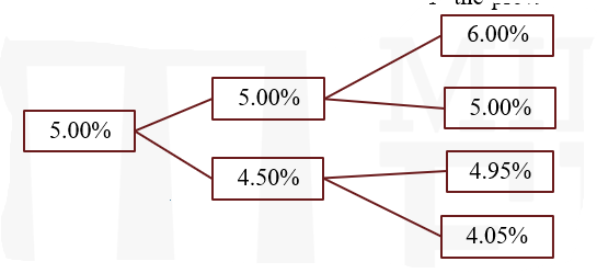
•When, as in this tree, an up move followed by a down move does not give the same rate as a   down move followed by an up move, the tree is said to be nonrecombining. From an economic   perspective, there is nothing wrong with this kind of tree. To justify this particular tree, for   example, one might argue that when short rates are 5% or higher, they tend to change in increments of 50 basis points. But when rates fall below 5%, the size of the change starts to decrease. In particular, at a rate of 4.50%, the short rate may change by only 45 basis points. A   volatility process that depends on the level of rates exhibits state-dependent volatility.

•The previous tree can be extended for the pricing of a 1.5-year zero assuming that the 1.5-year   spot rate is 5.25%. On date 3, the zero with an original term of 1.5 years matures and is worth   its face value of $1,000. On date 2, the value of the then six-month zero equals its face value discounted for six months at the then-prevailing spot rates of 6%, 5%, and 4% in states 2, 1, and 0, respectively:

Finally, on date 0, the 1.5-year zero equals its face value discounted at the given 1.5-year spot rate:

•The prices of the zero on date 1 in states 1 and 0 are denoted 𝑃_1,1 and 𝑃_1,0 respectively. The   then one-year zero prices are not known because, at this point in the development, possible   values of the one-year rate in six months are not available. Let 𝑞 be the risk-neutral probability   of an up move on date 1. By definition, expected discounted value under risk-neutral probabilities must produce market prices. With respect to the 1.5-year zero price on date 0, this requires that

With respect to the prices of a then 1-year zero on date 1,

•Furthermore, any derivative security that depends on the six-month rate in six months and in one year may be priced by computing its discounted expected value along this tree.

•The difference between the true and risk-neutral probabilities may once again be described in   terms of drift. From dates 1 to 2, the drift under the true probabilities is zero. Under the risk-   neutral probabilities the drift is computed from a 64.89% chance of a 50-basis point increase in   the six-month rate and a 35.11% chance of a 50-basis point decline in the rate. These numbers   give a drift or expected change of 14.89 basis points.

•To get the values of 𝑃_1,1 and 𝑃_1,0 𝑞 should be substituted as 0.6489 in the following

•So the complete tree for the price of the 1.5-year zero is given in this figure

•It follows immediately from this tree that the one-year spot  rate  six  months  from  now  may  be  either 5.5736% or 4.5743% Since

•The fact that the possible values of  the one-year spot rate can be extracted from the tree is at first surprising.

The starting point of the example is the date 0 values of the 0.5 —, 1 —, and 1.5-year spot rates as well as an assumption about the evolution of the six-month rate over the next year. But since this  information,  in  combination  with  arbitrage  or  risk-neutral  arguments,  is  sufficient  to determine the price tree of the 1.5-year zero, it is sufficient to determine the possible values of the one-year spot rate in six months.

Example: Pricing a Constant maturity Treasury Swap

•A constant maturity swap (CMS) is a variation of the regular interest rate swap in which the   floating portion of the swap is reset periodically against the rate of a fixed maturity instrument,   such as a Treasury note, with a longer maturity than the length of the reset period. In a regular or   vanilla swap, the floating portion is usually set against LIBOR, which is a short-term rate. A $1,000,000 face value of a stylized constant-maturity Treasury (CMT) swap struck at 5%, pays

every six months until it matures, where 𝑦_CMT  is a semiannually compounded yield, of  a

predetermined maturity, on the payment date. In practice, CMT swaps trade most commonly on the yields of the most liquid maturities, i.e., on 2 —, 5 — and 10 —year yields. Since six-month semiannually compounded yields equal six-month spot rates, rates from the tree of the previous section can be substituted to calculate the payoffs of the CMT swap.

On date 1, the state 1 payoff is $1,000,000 × 5.50%-5% / 2= $2,500

On date 1, the state 0 payoff is $1,000,000 × 4.50%-5% / 2= —$2500

On date 2, the state 2 payoff is $1,000,000 × 6%-5% / 2 = $5,000

On date 2, the state 1 payoff is $1,000,000 × 5%-5% / 2 = $0

On date 2, the state 0 payoff is $1,000,000 × 4%-5% / 2 = —$5,000

•The possible values of the CMT swap at maturity, on date 2, are given by the above payoffs. The   possible values on date 1 are given by the expected discounted value of the date 2 payoffs under   the risk-neutral probabilities plus the date 1 payoffs

On date 1, the state 1 value is :-

On date 1, the state 0 value is :-

The value of the swap on date 0 is the expected discounted value of the date 1 payoffs, under the risk-neutral probabilities which is

•This tree summarizes the value of the stylized CMT swap over dates and states. A value of $3,616.05 for the CMT swap might seem surprising at first. After all, the cash flows of the CMT swap are zero at a rate of 5%, and 5% is,under the real probabilities, the average rate on each date. The explanation, of course, is that the risk-neutral probabilities not the real probabilities, determine the arbitrage price of the swap. The expected discounted value of the swap under the real probabilities can be computed by following the same steps but using 0.5 for all up and down moves. The result of these calculations does give a value close to zero, namely —$5.80. The expected cash flow of the CMT swap on both dates 1 and 2,under the real probabilities, is zero. Hence, the discounted value of these expected cash flows is zero. At the same time, the expected discounted value of the CMT swap is —$5.80.

Option-Adjusted Spread

•Option-adjusted spread (OAS) is a widely-used measure of the relative value of a security, that is,   of its market price relative to its model value. OAS is defined as the spread such that the market   price of a security equals its model price when discounted values are computed at risk-neutral rates   plus that spread. To illustrate, let’s assume that the market price of the CMT swap in the previous   section is $3,613.25, $2.80 less than the model price. In that case, the OAS of the CMT swap   turns out to be 10 basis points. To see this, let’s add 10 basis points to the discounting rates of   5.5% and 4.5% in to get new swap values at date 1 of

Using the same OAS spread of 10 basis points, or 5.10%, the initial CMT swap value at date 0 is :-

Hence, as claimed, discounting at the risk-neutral rates plus an OAS of 10 basis points produces a model price equal to the given market price of $3,613.25.

•If a security’s OAS is positive, its market price is less than its model price, so the security trades cheap. If the OAS is negative, the security trades rich .

•Another perspective on the relative value implications of an OAS spread is the fact that the   expected return of a security with an OAS, under the risk-neutral process, is the short-term rate   plus the OAS per period. Very simply, discounting a security’s expected value by a particular rate   per period is equivalent to that security’s earning that rate per period.

•In the example of the CMT swap, the expected return of the fairly-priced swap under the risk-   neutral process over the six months from date 0 to date 1 is :-

which is six month’s worth of the initial rate of 5%.

•On the other hand, the expected return of the cheap swap, with an OAS of 10 basis points, is :-

which is six month’s worth of the initial rate of 5% plus the OAS of 10 basis points, or half of 5.10%.

Reducing The Time Step

•Till now, it has been assumed that the time elapsed between dates of the tree is 6 months. The methodology outlined previously, however, can be easily adapted to any time step of ∆𝑡 years. For monthly time steps, for example, ∆𝑡 =^1/12 or 0.0833, and one-month rather than six-month interest rates appear on the tree. Also, discounting must be done over the appropriate time interval. If  the rate of  term ∆𝑡 is 𝑟,then discounting means dividing by 1 + 𝑟∆𝑡 . In case of monthly time steps, discounting with a one-month rate of 5% means dividing by ( 1 + 0.05/12).

•In practice, there are two reasons to choose time steps smaller than six months.

1. First, a security or portfolio of securities rarely makes all of its payments in even six -month intervals from the starting date. Reducing the time step to a month, a week, or even a day can ensure that all cash flows are sufficiently close in time to some date in the tree.

2. Second, assuming that the six-month rate can take on only two values in six months, three values in one year, and so on, produces a tree that is too coarse for many practical pricing problems. Reducing the step size can fill the tree with enough rates to price contingent claims with sufficient accuracy.

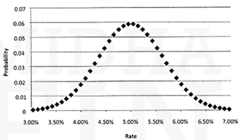
•This figure illustrates this point by showing   a  relatively  realistic-looking  probability   distribution of  the six-month rate in six   months from a tree with daily time steps, a   drift  of  zero,  and  a  horizon  standard   deviation of 65 basis points. While smaller   time steps generate more realistic interest   rate distributions, it is not the case that   smaller time steps are always desirable.

1. First, the greater the number of computations in pricing a security, the more attention must be paid to numerical issues like round-off error.

2. Second, since decreasing the time step increases computation time, practitioners requiring quick results cannot make the time step too small. Customers calling market makers in options on swaps, or swaptions, for example, expect price quotations within minutes if not sooner. Hence, the time step in a model used to price swaptions must be consistent with the market maker’s required response time.

•The best choice of step size ultimately depends on the problem at hand. When pricing a 30-year   callable bond, for example, a model with monthly time steps may provide a realistic enough   interest rate distribution to generate reliable prices. The same monthly steps, however, will   certainly be inadequate to price a one-month bond option: that tree would imply only two   possible rates on the option expiration date.

Fixed Income Versus Equity Derivatives

•Models created for the stock market cannot be adopted without modification for use in fixed   income markets. According to Black-Scholes-Merton pricing analysis of stock options – Under   the assumption that the stock price evolves according to a particular random process and that the   short-term interest rate is constant, it is possible to form a portfolio of stocks and short-term   bonds that replicates the payoffs of an option. Therefore, by arbitrage arguments, the price of   the option must equal the known price of the replicating portfolio.

•If an investor wants to price an option on a five- year bond by a direct application of this logic,   she investor would have to begin by making an assumption about how the price of the five-year   bond evolves over time. But this is considerably more complicated because

1. The price of a bond must converge to its face value at maturity while the random process describing the stock price need not be constrained in any similar way.

2. Because of the maturity constraint, the volatility of a bond’s price must eventually get smaller as the bond approaches maturity. The simpler assumption that the volatility of a stock is constant is not so appropriate for bonds.

3. Third, since stock volatility is very large relative to short-term rate volatility, it may be   relatively harmless to assume that the short-term rate is constant. By contrast, it can be difficult to defend the assumption that a bond price follows some random process while the short-term interest rate is constant.

•These objections led researchers to make assumptions about the random evolution of  the   interest rate rather than of the bond price. In that way bond prices would naturally approach par,   price volatilities would naturally approach zero, and the interest rate would not be assumed to be   constant. But this approach raises questions with regards to which interest rate should be   assumed to evolve in a particular way.

•Making assumptions about the 5-year rate over time is not particularly helpful for two reasons.

1. First, 5-year coupon bond prices depend on shorter-term rates as well.

2. Second, pricing an option on a 5-year bond requires assumptions about the bond’s future possible prices.

•But knowing the 5-year rate over time is insufficient because, in a very short time, the option’s   underlying security will no longer be a 5-year bond. Therefore, one must often make   assumptions about the evolution of the entire term structure of interest rates to price bond options and other derivatives.

•In the one-factor case described in this chapter it has been shown that modeling the evolution of   the short-term rate is sufficient, combined with arbitrage arguments, to build a model of the   entire term structure. In short, despite the enormous importance of  the Black-Scholes-Merton   analysis, the fixed income context does demand special attention.

Embedded Options In Fixed Income Securities

•A call option gives the issuer the right (but not the obligation) to buy back the bond at fixed   prices at one or more points in the future, prior to the date of maturity. The bondholder (or the   investor), by logic takes a short position in the call option. So the investor has the obligation to   sell the bond and  the right to purchase rests with the issuer. Compared to an option-free bond   which is identical in all other respects, this option reduces the value of the bond.

Value of a call option  =  value of option free bond – value of callable bond

⇒ Value of callable bond  =  value of option free bond — Value of the call option

•A put option gives the bondholder (or the investor) the right (but not the obligation) to sell the   bond back to the issuer at a set price. The issuer, by logic takes a short position in the put option.   So the issuer has the obligation to buy back the bond and  the right to sell rests with the   bondholder. Compared to an option-free bond which is identical in all other respects, this option   increases the value of the bond.

Value of a put option  = value of putable bond — value of option free bond

⇒ Value of putable bond  =  value of option free bond + Value of the put option