Challenges With Extreme Events

• Extreme events are events that are unlikely to occur, but can be very costly when they do. These events are often referred to as low-probability, high-impact events, and they include large market falls, the failures of major institutions, the outbreak of financial crises and natural catastrophes. There are many problems in risk management that deal with extreme events –
1. There are relatively few extreme observations available on which to base our estimates. This is why estimates of extreme risks are very uncertain, and this uncertainty is especially pronounced if extreme risks have to be considered not only within the range of observed data, but well beyond the historical data set (e.g., an unprecedented stock market fall).
2. Practitioners can only respond by relying on assumptions to make up for lack of data. Unfortunately, the assumptions they make are often questionable. Typically, a distribution is selected arbitrarily, and then fitted to the whole data set. However, this means that the fitted distribution will tend to accommodate the more central observations, because there are so many of them, rather than the extreme observations, which are much sparser. Hence, this type of approach is often good if we are interested in the central part of the distribution, but is not suited for handling extremes.
3. EVT focuses on the distinctiveness of extreme values and makes use of a lot of theory. EVT is quite different from the more familiar ‘central tendency’ statistics. Not only the EV distributions, but their parameters are also different, and the estimation of these parameters is more difficult.

Generalised Extreme-Value Theory

• Consider a random loss variable X, which is independent and identically distributed (iid) from some unknown distribution F(x)=Prob(X ≤ x). The estimation of extreme risks (e.g., extreme VaR) associated with the distribution of X is not easy because F(x) is not known.
• This is where EVT can help. Consider a sample of size n drawn from F(x), and let the maximum of this sample be M_n If n is large, M_n can be regarded as an extreme value. Under relatively general conditions, Fisher-Tippett theorem (1928) then tells us that as n gets large, the distribution of extremes (i.e., M_n) converges to the following generalized extreme-value (GEV) distribution:



where  x satisfies the condition 1+ξ (x-μ)/σ > 0.

• This distribution has three parameters:
1. μ, the location parameter of the limiting distribution, which is a measure of the central tendency of M_n, and
2. σ, the scale parameter of the limiting distribution, a measure of the dispersion of M_n.
3. ξ, the tail index, gives an indication of the shape (or heaviness) of the tail of the limiting distribution.
• The GEV Equation has three special cases:
1. If ξ>0, the GEV becomes the Frechet distribution, where the tail of F(x) obeys a power function and is therefore heavy (e.g., as would be the case if F(x) were a Levy distribution, a t-distribution, a Pareto distribution, etc.). This case is particularly useful for financial returns because they are typically heavy tailed, and we often find that estimates of ξ for financial return data are positive but less than 0.35.
2. If ξ=0, the GEV becomes the Gumbel distribution, where F(x) has exponential tails. These are relatively light tails such like normal or lognormal distributions.
3. If ξ<0, the GEV becomes the Weibull distribution, where F(x) has lighter than normal tails. However, the Weibull distribution is not particularly useful for modelling financial returns, because few empirical financial returns series are so light-tailed.
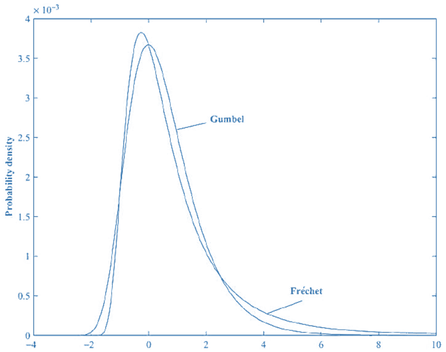
• The standardised (i.e., μ = 0, σ = 1) Frechet and Gumbel probability density functions are illustrated in this figure. Both are skewed to the right, but the Frechet is more skewed than the Gumbel and has a noticeably longer right-hand tail. This means that the Frechet has considerably higher probabilities of producing very large X-values.
• Most of the probability mass is located between x values of -2 and +6. More generally, this means most of the probability mass will lie between x values of μ-2σ and μ+6σ.



• There are various ways to decide which EV distribution to use:
1. If there is confidence that the parent loss distribution can be identified, the EV distribution can be chosen in whose domain of attraction the parent distribution resides. For example, If there is confidence that the parent loss distribution is a t-distribution, then the Frechet distribution should be chosen, because the t-distribution belongs in the domain of attraction of the Frechet.
2. The significance of the tail index could be tested, and the Gumbel might be chosen if the tail index was insignificant and the Frechet otherwise. However, this leads to the danger that ξ might be incorrectly concluded to be 0, and this could lead to underestimation of extreme risk measures.
3. Given the dangers of model risk and bearing in mind that the estimated risk measure increases with the tail index, a safer option is always to choose the Frechet.

A Short-Cuv Ev Method

• There are also short-cut ways to estimate VaR (or ES) using EV theory. These are based on the idea that if ξ > 0, the tail of an extreme loss distribution follows a power-law times a slowly varying function:



where  k(x) varies slowly with x.

For example, if it is assumed for convenience that k(x) is approximately constant, then



• Now consider two probabilities, a first, ‘in-sample’ probability P_in-sample and a second, smaller and typically ‘out-of-sample’ probability P_{out-of-sample}.









• This allows to estimate one quantile (denoted here as x_{out-of-sample} based on a known in-sample quantile x_in-sample  a known out-of-sample probability P_{out-of-sample} (which is known because it comes directly from the VaR confidence level), and an unknown in-sample probability P_in-sample  · The latter can easily be proxied by its empirical counterpart, t/n,  where n is the sample size and t the number of observations higher than x_(in-sample)  · Using this proxy

The Peaks-Over-Threshold Approach: The Generalized Pareto Distribution

• This approach deals with the application of EVT to the distribution of excess losses over a (high) threshold. The peaks-over-threshold (POT) or generalized Pareto approach, (generally) requires fewer parameters than EV approaches based on the generalized extreme value theorem. The POT approach provides the natural way to model exceedances over a high threshold, in the same way that GEV theory provides the natural way to model the maxima or minima of a large sample.
• If X is a random iid loss with distribution function F(x), and u is a threshold value of X, the distribution of excess losses over the threshold u can be defined as:



This gives the probability that a loss exceeds the threshold u by at most x, given that it does exceed the threshold. The distribution of X itself can be any of the commonly used distributions: normal, lognormal, t, etc., and will usually be unknown. However, as u gets large, the Gnedenko-Pickands-Balkema-deHaan (GPBdH) theorem states that the distribution F_u (x) converges to a generalized Pareto distribution, given by:



defined for

x ≥ 0 for ξ ≥ 0, and

0 ≤ x ≤β/ξ for ξ < 0.

This distribution has only two parameters: a positive scale parameter, β, and a shape or tail index parameter, ξ , that can be positive, zero or negative. This latter parameter is the same as the tail index encountered already with GEV theory. ξ > 0 corresponds to data being heavy tailed.

• The GPBdH theorem is a very useful result, because it states that the distribution of excess losses always has the same form (in the limit, as the threshold gets high), pretty much regardless of the distribution of the losses themselves. Provided the threshold is high enough,  the GP distribution should be regarded as the natural model for excess losses.
• To apply the GP distribution, a reasonable threshold u needs to be chosen, which determines the number of observations, N_u, in excess of the threshold value. Choosing u involves a trade-off:
1. u to be sufficiently high for the GPBdH theorem to apply reasonably closely
2. but if u is too high, there won’t be enough excess-threshold observations on which to make reliable estimates.
• The parameters ξ and β also need to be estimated. As with the GEV distributions, we can estimate these using maximum likelihood approaches or semi-parametric approaches.
• Now using some algebra, the following equations can be obtained



where  x > u.



• The VaR is given by the x-value is given by



where  α, is the VaR confidence level.

• The ES is then equal to the VaR plus the mean-excess loss over VaR. Provided ξ < 1,

Gev vs Pot

• Both GEV and POT approaches are different manifestations of the same underlying EV theory, although GEV is geared towards the distribution of extremes as such, whereas POT other is geared towards the distribution of exceedances over a high threshold. In theory, there is therefore not too much to choose between them, but in practice there may sometimes be reasons to prefer one over the other:
1. One might be more natural in a given context than the other (e.g., limited data  would make one preferable).
2. The GEV typically involves an additional parameter relative to the POT, and the most popular GEV approach, the block maxima approach (which has been implicitly assumed so far), can involve some loss of useful data relative to the POT approach, because some blocks might have more than one extreme in them. Both of these are disadvantages of the GEV relative to the POT.
3. On the other hand, the POT approach has to deal with the problem of choosing the threshold, and this problem does not arise with the GEV.

Refinements To Ev Approaches

• These fall under three headings:
1. Conditional EV.
2. Dealing with dependent (or non-iid) data.
3. Multivariate EVT.

MultiVariate Evt

• Multivariate extreme value theory (MEVT) can be used to model the tails of multivariate distributions in a theoretically appropriate way. The key issue here is how to model the dependence structure of extreme events. To appreciate this issue, it is again important to recognize how EV theory differs from more familiar central-value theory. When dealing with central values, the central limit theorem is used to justify the assumption of a normal (or more broadly, elliptical) distribution. With such a distribution, the dependence structure can then be captured by the (linear) correlations between the different variables. Given the distributional assumptions, knowledge of variances and correlations (or, if we like, covariances) suffices to specify the multivariate distribution. This is why correlations are so important in central-value theory. .
• However, this logic does not carry over to extremes. Beyond elliptical distributions, correlation no longer is sufficient to describe the dependence structure. Instead, the modeling of multivariate extremes requires the use of copulas. MEVT states that the limiting distribution of multivariate extreme values will be a member of the family of EV copulas, and multivariate EV dependence can be modelled by assuming one of these EV copulas. In theory, such copulas can also have as many dimensions as required, reflecting the number of random variables to be considered. However, there is a curse of dimensionality here. For example, if there are two independent variables and univariate extreme events are classified as those that occur one time in a 100, then one multivariate extreme event (i.e., both variables taking extreme values) is expected to be only one time in 100² , or one time in 10,000 observations; with three independent variables, one multivariate extreme event is expected to be one time in 100³ , or one time in 1,000,000 observations, and so on. As the dimensionality rises, the multivariate EV events rapidly become much rarer: there are fewer multivariate extreme observations to work with, and more parameters to estimate. There is clearly a limit to how many dimensions that can be handled.

From this example, it should not be concluded mistakenly that multivariate extremes are sufficiently rare and not of much concern. Extreme events cannot be assumed to be independent but their occurrence is governed by the tail dependence of the multivariate distribution. Hence, tail dependence is the central focus of MEVT. And, as a matter of empirical fact as well, extreme events are not independent. For example – a major earthquake can trigger other natural or financial disasters (e.g., tsunamis or market crashes).