Introduction

• The essence of non-parametric approaches  is that we try to let the P/L data speak for themselves as much as possible, and use the recent empirical (or in some cases simulated) distribution of P/L – not some assumed theoretical distribution – to estimate our risk measures.
• All non-parametric approaches are based on the underlying assumption that the near future will be sufficiently like the recent past. In deciding whether to use any non-parametric approach, it is important to form a conclusion regarding the extent to which data from the recent past will be a good guide about the risks faced over the relevant time horizon.
• The most popular non-parametric approach-historical simulation (HS). Loosely speaking, HS is a histogram-based approach. it is
  
  • conceptually simple,
  • easy to implement,
  • very widely used, and
  • has a fairly good historical record.
•   Refinements can be made to basic HS using bootstrap and kernel methods.

Bootstrapped Historical Simulation

• One simple but powerful improvement over basic HS is to estimate VaR and ES from bootstrapped data. A bootstrap procedure involves resampling from the existing data set with replacement.
  • Each new ‘resampled’ sample gives a new VaR estimate, and the ‘best’ estimate can be taken as the mean of these resample-based estimates.
  • The same approach can also be used to produce resample-based ES estimates.
• A bootstrapped estimate will often be more accurate than a ‘raw’ sample estimate.
• Bootstraps are also useful for gauging the precision of the estimates.

HS Using Non-Parametric Density Estimation

• HS does not make the best use of information. It also has the practical drawback that it only allows to estimate VaRs at discrete confidence intervals determined by the size of the data set.
  • For example, if there are 100 HS P/L observations, basic HS does not allow the estimation of VaR at the 95.1% confidence level, because there is no corresponding loss observation to go with it.
  • It should be greater than the sixth largest loss (or the 95% VaR), and smaller than the fifth largest loss (or the 96% VaR), but with only 100 observations there is no observation that corresponds to any VaR whose confidence level involves a fraction of 1%.
  • Hence, with n observations, basic HS only allows to estimate the VaRs associated with, at best, n different confidence levels.

• Non-parametric density estimation offers a potential solution to both these problems. The idea is to treat our data as if they were drawings from some unspecified or unknown empirical distribution function. This approach also encourages us to confront potentially important decisions about the width of bins and where bins should be centered, and these decisions can sometimes make a difference to our results.
• Non-parametric density estimation allows the estimation of VaRs and ESs for any confidence levels and so constraints imposed by the size of the data set can be avoided. In effect, it enables drawing lines through points on or near the edges of the ‘bars’ of a histogram. The areas under these lines can then be treated as a surrogate PDF, and so proceed to estimate VaRs for arbitrary confidence levels.
• A simple way to do this is to draw in straight lines connecting the mid-points at the top of
  each histogram bar, as illustrated in the figure. Once these lines are drawn, the histogram bars can be ignored and the area under the lines can be treated as a PDF. This enables the estimation of VaRs at any confidence level, regardless of the size of the data set.

• Notice that by connecting the midpoints, the upper portion gains some area and the lower portion loses an equal amount of area. So overall, no area is lost, only displaced.
• Of course, drawing straight lines through the mid-points of the tops of histogram bars is not the best option. Smooth curves can also be drawn that meet up nicely, and so on.
• Besides using a histogram, data can also be represented using naive estimators or kernels, which are generally superior.

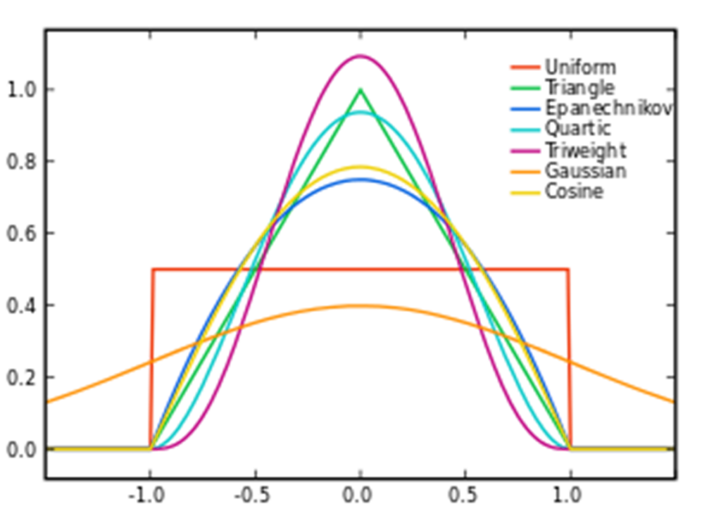
Brian Amberg [CC BY-SA 3.0 (https://creativecommons.org/licenses/by-sa/3.0)]

• Research suggests that the different types of kernel methods produce quite similar VaR estimates, although to the extent that there are differences among them, they also found that the ‘best’ kernels were the adaptive Epanechinikov and adaptive Gaussian ones.
• Although kernel methods are better in theory, they do not necessarily produce much better estimates in practice. Crude methods like drawing straight-line ‘curves’ through the tops of histograms are more transparent and easier to check.

Equal weighted Historical Simulation – Issues

• One of the most important features of traditional HS is the way it weights past observations. In the basic HS approach, observations up to a specified cutoff period are used and all have equal weights. So if the total number of observations is n, our HS P/L series is constructed in a way that gives any observation the same weight (=1/n) on P/L which is less than n periods old, and no weight (i.e., a zero weight) if it is older than that.
• This weighting structure has a number of problems.
  
  1.  One problem is that it is hard to justify giving each observation in our sample period the same weight, regardless of age, market volatility, or anything else. A good example of the difficulties this can create is given by Shimko et. al. (1998). It is well known that natural gas prices are usually more volatile in the winter than in the summer, so a raw HS approach that incorporates both summer and winter observations will tend to average the summer and winter observations together. As a result, treating all observations as having equal weight will tend to underestimate true risks in the winter, and overestimate them in the summer.
  2. The equal-weight approach can also make risk estimates unresponsive to major events. For instance, a stock market crash might have no effect on VaRs except at a very high confidence level, so we could have a situation where everyone might agree that risk had suddenly increased, and yet that increase in risk would be missed by most HS VaR estimates. The increase in risk would only show up later in VaR estimates if the stock market continued to fall in subsequent days. The increase in risk would show up in ES estimates just after the first shock occurred—which is, incidentally, a good example of how ES can be a more informative risk measure than the VaR.
  3. The equal-weight structure also presumes that each observation in the sample period is equally likely and independent of the others over time. However, this ‘iid’ assumption is unrealistic because it is well known that volatilities vary over time, and that periods of high and low volatility tend to be clustered together.
  4. It is also hard to justify why an observation should have a weight that suddenly goes to zero when it reaches age n. Why is it that an observation of age n – 1 is regarded as having a lot of value (and, indeed, the same value as any more recent observation), but an observation of age n is regarded as having no value at all?
  5. Also, giving zero weights to old observations tends to violate the old statistical adage that information should never be thrown away.
  6. This weighting structure also creates the potential for ghost effects – we can have a VaR that is unduly high (or low) because of a small cluster of high loss observations, or even just a single high loss, and the measured VaR will continue to be high (or low) until n days or so have passed and the observation has fallen out of the sample period. At that point, the VaR will fall again, but the fall in VaR is only a ghost effect created by the weighting structure and the length of sample period used.

To address these issues, we can use ‘weighted historical simulation’ which can be regarded as semi-parametric methods because they combine features of both parametric and non-parametric methods.

Age Weighted Historical Simulation

• This approach is to weight the relative importance of the observations by their age. Their probabilities can be weighted so as to discount the older observations in favor of newer ones.

  • Thus, if w(1) is the probability weight given to an observation 1 day old, then

    • w(2), the probability given to an observation 2 days old, could  be λw(1);

    • w(3) could be λw(2)=λ^2 w(1);

      and so on.

      The λ term is between 0 and 1, and reflects the exponential rate of decay in the weight or value given to an observation as it ages. A λ close to 1 indicates a slow rate of decay, and a λ far away from 1 indicates a high rate of decay.

• This age-weighted approach has four major attractions –

• 1. First, it provides a nice generalization of traditional HS, because we can regard traditional HS as a special case with zero decay, or λ→1.

  2. Second, a suitable choice of λ can make the VaR (or ES) estimates more responsive to recent large loss observations, and they are also better at handling clusters of large losses.

  3. Third, age-weighting helps to reduce distortions caused by events that are unlikely to recur, and helps to reduce ghost effects. As an observation ages, its probability weight gradually falls and its influence diminishes gradually over time. Furthermore, when it finally falls out of the sample period, its weight will fall from to zero, instead of from 1/n to zero. Since λ^n w(1) is less than 1/n for any reasonable values of X and n, then the shock – the ghost effect – will be less than it would be under equal-weighted HS.

  4. Since age-weighting allows the impact of past extreme events to decline as past events recede in time, it gives us the option of letting the sample size grow over time. This means that potentially valuable information is never thrown away. This would improve efficiency and eliminate ghost effects even further, because there would no longer be any ‘jumps’ in the sample resulting from old observations being thrown away.

Volatility Weighted Historical Simulation

• The data can also be weighted by volatility. The basic idea is to update return information to take account of recent changes in volatility.
  • For example, if the current volatility in a market is 1.5% a day, and it was only 1% a day a month ago, then one month old would underestimate tomorrow’s risks.
  • On the other hand, if last month’s volatility was 2 % a day, then month-old data would overestimate tomorrow’s risks.

    So, the historical returns should be adjusted to reflect how volatility tomorrow is believed to have changed from its past values.

• Suppose the VaR for day T has to be forecasted. Let r_(t,i) be the historical return for the i^th asset on day t in the historical sample, and σ_(t,i) be the historical GARCH (or EWMA) forecast of the volatility of the return on that i^th asset for day t, made at the end of day t-1, and σ_(T,i) be the most recent forecast of the volatility of that i^th asset. The volatility-adjusted returns will be given by

\[ r_{(t,i)}^* = \frac{\sigma_{(T,i)}}{\sigma_{(t,i)}} \times r_{(t,i)} \]

• Actual returns in any period t are therefore increased (or decreased), depending on whether the current forecast of volatility is greater (or less than) the estimated volatility for period t. The HS P/L is now calculated using the volatility-adjusted returns and then HS VaRs or ESs are estimated in the traditional way (i.e., with equal weights, etc.)
• This approach has several advantages relative to the traditional equal-weighted and/or the age-weighted approaches –
  

  • It takes account of volatility changes in a natural and direct way, whereas equal-weighted HS ignores volatility changes, and the age-weighted approach treats volatility changes in a rather arbitrary and restrictive way.

  • It produces risk estimates that are appropriately sensitive to current volatility estimates, and incorporates information from GARCH forecasts into HS VaR and ES estimation.

  • It allows to obtain VaR and ES estimates that can exceed the maximum loss in the historical data set. In periods of high volatility, historical returns are scaled upwards, and the HS P/L series used in this procedure will have values that exceed actual historical losses. This is a major advantage over traditional HS, which prevents the VaR or ES from being any bigger than the losses in the historical data set.

  • Empirical evidence indicates that this approach produces superior VaR estimates to the age-weighted approaches.

Correlation Weighted Historical Simulation

• The historical returns can also be adjusted to reflect changes between historical and current correlations. The historic returns are multiplied by the revised correlation matrix to yield updated correlation-adjusted returns.
• This approach gives a weighting system that takes account of updated correlations as well as volatilities.

Filtered Historical Simulation(FHS)

• Another promising but complex approach is filtered historical simulation (FHS). This is a form of semi-parametric bootstrap which aims to combine the benefits of HS with the power and flexibility of conditional volatility models such as GARCH. 

  This is achieved by bootstrapping returns within a conditional volatility (e.g., GARCH) framework, where –

  • the bootstrap preserves the non-parametric nature of HS, and

  • the volatility model gives a sophisticated treatment of volatility.

• For estimating VaR of a single-asset portfolio over a 1-day holding period, the following steps are followed –
  1. A conditional volatility model like GARCH is fitted to the portfolio-return data. It has been recommended to use an asymmetric GARCH, or AGARCH, model. This allows positive and negative returns to have differential impacts on volatility, a phenomenon known as the leverage effect. For a multi-asset portfolio, a multivariate AGARCH would be used.
  2. The second step is to use the model to forecast volatility for each of the days in a sample period. These volatility forecasts are then divided into the realized returns to produce a set of standardized returns. These standardized returns should be i.i.d. to be suitable for HS.

  3. The third stage involves bootstrapping from the data set of standardized returns. Assuming a 1-day VaR holding period, the simulated returns, are scaled by today’s forecast of tomorrow’s volatility.

  4. Finally, the VaR is calculated as the loss corresponding to the chosen confidence level.

• FHS has a number of attractions –
  

  1. It combines the non-parametric attractions of HS with a sophisticated (e.g., GARCH) treatment of volatility, and so takes account of changing market volatility conditions

  2. It is fast, even for large portfolios.

  3. allows for VaR and ES estimates to exceed the maximum historical loss in the data set.

  4. It maintains the correlation structure in the return data without relying on knowledge of the variance-covariance matrix or the conditional distribution of asset returns

  5. It can be modified to take account of autocorrelation or past cross-correlations in asset returns

  6. It can be modified to produce estimates of VaR or ES confidence intervals by combining it with an OS or bootstrap approach to confidence interval estimation

  7. There is evidence that FHS works well.

Advantages of Non-Parametric Methods

1. Non-parametric approaches are intuitive and conceptually simple.
2. Since they do not depend on parametric assumptions about P/L, they can accommodate fat tails, skewness, and any other non-normal features that can cause problems for parametric approaches.
3. They can in theory accommodate any type of position, including derivatives positions.
4. There is a widespread perception among risk practitioners that HS works quite well empirically, although formal empirical evidence on this issue is inevitably mixed.
5. They are (in varying degrees, fairly) easy to implement on a spreadsheet.
6. Non-parametric methods are free of the operational problems to which parametric methods are subject when applied to high-dimensional problems – no need for covariance matrices, no curses of dimensionality, etc.
7. They use data that are (often) readily available, either from public sources (e.g., Bloomberg) or from in-house data sets (e.g., collected as a by-product of marking positions to market).
8. They provide results that are easy to report and communicate to senior managers and interested outsiders (e.g., bank supervisors or rating agencies).
9. It is easy to produce confidence intervals for nonparametric VaR and ES.
10. Non-parametric approaches are capable of considerable refinement and potential improvement if they are combined with parametric ‘add-ons’ to make them semi-parametric. Such refinements include age-weighting, volatility-weighting, and correlation-weighting.

Disadvantages of Non-Parametric Methods

1. If the data period was unusually quiet, non-parametric methods will often produce VaR or ES estimates that are too low, and if the data period was unusually volatile, they will often produce VaR or ES estimates that are too high.
2. Non-parametric approaches can have difficulty handling shifts that take place during the sample period. For example, if there is a permanent change in exchange rate risk, it will usually take time for the HS VaR or ES estimates to reflect the new exchange rate risk. Similarly, such approaches are sometimes slow to reflect major events, such as the increases in risk associated with sudden market turbulence.
3. If the data set incorporates extreme losses, these losses can dominate nonparametric risk estimates even though they are not expected to recur.
4. Most non-parametric methods are subject to the phenomenon of ghost or shadow effects.
5. In general, non-parametric estimates of VaR or ES make no allowance for plausible events that might occur, but did not actually occur, in our sample period.
6. Non-parametric estimates of VaR and ES are to a greater or lesser extent constrained by the largest loss in the historical data set. More sophisticated versions of HS can relax this constraint, but still, it does not get fully unconstrained like parametric estimates. This means that such methods are not well suited to handling extremes, particularly with small- or medium-sized samples.

• However, with these problems can be managed by suitable refinements. For example, volatility, market turbulence, correlation and other problems can be dealt by semi-parametric adjustments, and ghost effects can be dealt by age-weighting.
  1.