Introduction

•A fairly recent and famous as well as infamous correlation approach applied in finance is the  copula approach.

•When flexible copula functions were introduced to finance in 2000, they were enthusiastically  embraced but then fell into disgrace when the global financial crisis hit in 2007.

•Copulas became popular because they could presumably solve a complex problem in an easy  way: It was assumed that copulas could correlate multiple assets, for example the 125 assets in a  CDO, with a single (although multidimensional) function.

•There are benefits and limitations of the Gaussian copula for valuing CDOs.

Copula Correlations

•Copula functions are designed to simplify statistical problems. They allow the joining of multiple  univariate distributions to a single multivariate distribution. Formally, a copula function C transforms  an n-dimensional function on the interval [0, 1] into a unit-dimensional one:

More generally, let 𝐺_i  𝑢_i  𝜖[0,1] be a univariate, uniform distribution with 𝑢_i = 𝑢₁ ….. 𝑢_n, and

𝑖 𝜖 𝑁. Then there exists a copula function C such that

where 𝐺_i  𝑢_i  are called marginal distributions, 𝐹_n  is the joint cumulative distribution function 𝐹^–1 is the inverse of 𝐹_i, and 𝜌_F is the correlation structure of 𝐹_n.

This equation can be read as :

Given are the marginal distributions 𝐺₁ 𝑢₁  𝑡𝑜 𝐺_n 𝑢_n  .

There  exists  a  copula  function  that  allows  the  mapping  of  the  marginal  distributions 𝐺₁ 𝑢₁  𝑡𝑜 𝐺_n  𝑢_n  via 𝐹^–1 and the joining of the (abscise values) 𝐹^–1(𝐺_i(𝑢_i)) to a single, n-variate function 𝐹_n  𝐹^–1  𝐺₁ 𝑢₁  …., 𝐹^–1  𝐺_n  𝑢_n  with correlation structure of 𝜌_F.

If the mapped values 𝐹^–1  𝐺_i  𝑢_i are continuous, it follows that 𝐶 is unique.

Types of Copula Function

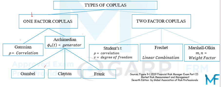
Numerous types of copula functions exist. They can be broadly categorized in one-parameter  copulas as the Gaussian copula and the Archimedean copula family, the most popular being  Gumbel, Clayton, and Frank copulas. Often cited two-parameter copulas are Student’s t, Frechet,  and Marshall-Olkin. This figure shows an overview of popular copula functions.

The Gaussian Copula

•Due to its convenient properties, the Gaussian copula 𝐶_G is among the most applied copulas  in finance. In the n-variate case, it is defined

𝐶_G [𝐺₁(𝑢₁),…., 𝐺_n(𝑢_n)]  = 𝑀_n[𝑁^–1(𝐺₁(𝑢₁)), …  , 𝑁^–1(𝐺_n(𝑢_n)); 𝜌_M]

where

𝑀_n is the joint, 𝑛-variate cumulative standard normal distribution

𝜌_M, the 𝑛× 𝑛 symmetric, positive-definite correlation matrix of the n-variate normal  distribution 𝑀_n.

𝑁^–1 𝑖𝑠 the inverse of a univariate standard normal distribution.

If the 𝐺_x(𝑢_x) are uniform, then the 𝑁^–1(𝐺_x(𝑢_x)) are standard normal and 𝑀_n is standard  multivariate normal.

•It was David Li (2000) who transferred the Gaussian copula approach to finance. He defined the  cumulative default probabilities 𝑄 for entity 𝑖 at a fixed time 𝑡, 𝑄(𝑡) as marginal distributions.  Hence, the Gaussian default time copula 𝐶_GD can be derived as

This equation reads: Given are the marginal distributions, that is, the cumulative default  probabilities 𝑄 of entities 𝑖  = 1 to 𝑛 at times 𝑡, 𝑄_i(𝑡). There exists a Gaussian copula function

𝐶_GD, which allows the mapping of the marginal distributions 𝑄_i  𝑡  via 𝑁^–1 to standard normal

and the joining of the (abscise values) 𝑁^–1𝑄_i(𝑡) to a single 𝑛-variate standard normal  distribution 𝑀_n with the correlation structure 𝜌_M.

More precisely, the term 𝑁^–1 maps the cumulative default probabilities 𝑄 of asset 𝑖 for time 𝑡,

𝑄_i(𝑡), percentile to percentile a univariate standard normal distribution. So the 5th percentile of

𝑄_i(𝑡) is mapped to the 5th percentile of the standard normal distribution, the 10th percentile of

𝑄_i(𝑡) is mapped to the 10th percentile of the standard normal distribution, and so forth. As a result, the 𝑁^–1(𝑄_i 𝑡 ) in the above equation are abscise (x-axis) values of the standard normal  distribution. The 𝑁^–1(𝑄_i(𝑡)) are then joined to a single 𝑛-variate distribution 𝑀_n by applying  the correlation structure of the multivariate normal distribution with correlation matrix 𝜌_M. The probability of 𝑛 correlated defaults at time 𝑡 is given by 𝑀_n.

•Graphically the mapping 𝑁^–1(𝑄(𝑡)) can be  represented in two steps, which are displayed in this  figure. In the lower graph, the cumulative default  probability of company 𝐵, 𝑄_B 𝑡 , is displayed. First,  these cumulative probabilities are mapped percentile  to percentile to a cumulative standard normal  distribution in the upper graph (up arrows). In a second  step  the  abscise  (x-axis) values of  the cumulative  normal  distribution  are found (down arrows).

•The same mapping procedure is done for company 𝐶𝑎𝑎; the cumulative default probabilities of company 𝐶𝑎𝑎 ,  are  mapped  percentile to  percentile  to  a cumulative  standard  normal distribution  via 𝑁^–1(𝑄_Caa(𝑡)).

•Importantly, the copula model now assumes that we can apply the correlation structure 𝜌_M or  a single 𝜌 of the multivariate distribution (in our case the Gaussian multivariate distribution M)  to the transformed marginal distributions 𝑁^–1(𝑄_B(𝑡)) 𝑎𝑛𝑑 𝑁^–1(𝑄_Caa(𝑡)). This is done for  mathematical and computational convenience.

Now the joint default probabilities of the companies 𝐵 and 𝐶𝑎𝑎 can be found out by using  the bivariate cumulative distribution

For example,

The joint default probability 𝑄 of companies 𝐵 and 𝐶𝑎𝑎 in the next year assuming a one-year  Gaussian default correlation of 0.4 is:

𝑄 𝑡_B ≤ 1 ∩ 𝑡_caa ≤ 1  ≡ 𝑀(𝑥_B ≤ —1.5133 ∩ 𝑥_caa ≤ —0.7118, 𝜌 = 0.4) = 3.44%

where 𝑡_B is the default time of company Band 𝑡_caa is the default time of company Caa. 𝑥_B

and 𝑥_caa are the mapped abscise values of the bivariate normal distribution.

Another example –

The joint probability of company 𝐵 defaulting in year 3 and company 𝐶𝑎𝑎 defaulting in year 5  is

𝑄 𝑡_B ≤ 3 ∩ 𝑡_caa ≤ 5  ≡ 𝑀(𝑥_B ≤ —0.8054 ∩ 𝑥_caa ≤ —0.2557, 𝜌 = 0.4) = 16.93%

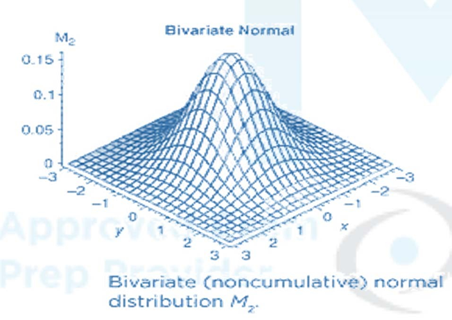
The bivariate normal distribution 𝑀₂ is displayed in this figure.

The code for the bivariate cumulative normal distribution M can be found on the Internet

The Gaussian Copula-Example

•Let’s assume we have two companies, 𝐵 and 𝐶𝑎𝑎, with their estimated default probabilities for  year 1 to 10 as displayed in this table. Default probabilities for investment grade companies  typically increase in time, since uncertainty increases with time. However, in this table, there are  two companies currently in distress. For these companies the next few years will be the most  difficult. If they survive these next years, their default probability will decrease.

Default Probability and Cumulative Default Probability of Companies B and Caa

Default Time t	Company B Default Probability	Company B Cumulative Default Probability \(Q_B(t)\)	Company Caa Default Probability	Company Caa Cumulative Default Probability (Q_{Caa}(t)
1	6.51%	6.51%	23.83%	23.83%
2	7.65%	14.16%	13.29%	37.12%
3	6.87%	21.03%	10.31%	47.43%
4	6.01%	27.04%	7.62%	55.05%
5	5.27%	32.31%	5.04%	60.09%
6	4.42%	36.73%	5.13%	65.22%
7	4.24%	40.97%	4.04%	69.26%
8	3.36%	44.33%	4.62%	73.88%
9	2.84%	47.17%	2.62%	76.50%
10	2.84%	50.01%	2.04%	78.54%

Let’s now find the joint default  probabilities of  the companies 𝐵and 𝐶𝑎𝑎 for any time 𝑡 with  the Gaussian copula function ,  First the cumulative default  probabilities 𝑄 𝑡 (which are in  columns 3 and 5 in this table)  are mapped to the standard  normal distribution via 𝑁^–1(𝑄(𝑡)).

•The percentile to percentile mapped cumulative default probability values of our companies to  cumulative standard normal distribution (𝑁^–1(𝑄_B(𝑡)) and 𝑁^–1(𝑄_caa(𝑡))) are displayed in this  table, columns 3 and 5. Since 𝑛  = 2 companies in our example, we can write

Cumulative Default Probabilities and Corresponding Standard Normal Percentiles of Companies B and Caa

Default Time \(t\)	Company B Cumulative Default Probability \(Q_B(t)\)	Company B Cumulative Standard Normal Percentiles \(N^{-1}(Q_B(t))\)	Company Caa Cumulative Default Probability \(Q_{Caa}(t)\)	Company Caa Cumulative Standard Normal Percentiles \(N^{-1}(Q_{Caa}(t))\)
1	6.51%	-1.5133	23.83%	-0.7118
2	14.16%	-1.0732	37.12%	-0.3287
3	21.03%	-0.8054	47.43%	-0.0645
4	27.04%	-0.6116	55.05%	0.1269
5	32.31%	-0.4590	60.09%	0.2557
6	36.73%	-0.3390	65.22%	0.3913
7	40.97%	-0.2283	69.26%	0.5032
8	44.33%	-0.1426	73.88%	0.6397
9	47.17%	-0.0710	76.50%	0.7225
10	50.01%	0.0003	78.54%	0.7906

Simulating the Correlated Default Time for Multiple Assets

•To derive the default time of asset 𝑖, 𝜏_i, which is correlated to the default times of  all other  assets  𝑖  =  1, …  , 𝑛 ,  first,  a  sample  𝑀_n   ·  from  a  multivariate  copula  is  derived,  where 𝑀_n (·) 𝜖 [0,1]  .  This  is  done  via  Cholesky  decomposition.  The  sample  includes  the  default  correlation via the default correlation matrix 𝜌_M of the 𝑛-variate standard normal distribution 𝑀_n. Then the sample(·) from 𝑀_n (which is 𝑀_n(·)) is equated with the cumulative individual  default probability 𝑄 of asset 𝑖 at time 𝜏, 𝑄_i(𝜏_i). Therefore,

•There is no closed-form solution for the above equations. To find the solution, a search  procedure such as Newton-Raphson can be used. It can also be done use a simple lookup  function in Excel.

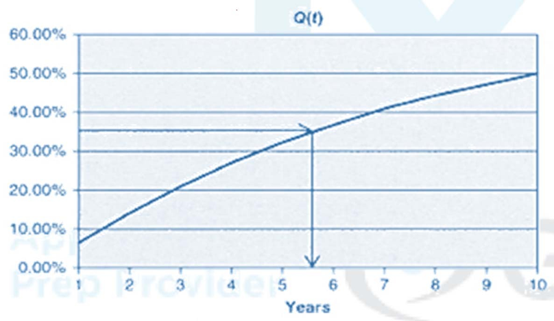
•Let’s assume the random drawing from 𝑀_n(·) was 35%. Now 35% is equated with the market  given function 𝑄_i(𝜏_i) and the expected default time 𝜏_i of asset 𝑖, is found out. This is displayed  in this figure, where 𝜏_i = 5.5 years. This procedure is repeated numerous times, for example  100,000 times, and each 𝜏_i of every simulation is averaged to obtain the estimate for 𝜏_i  Importantly, the estimated default time 𝜏_i of asset 𝑖, includes the default correlation with the  other assets in the portfolio, since the correlation matrix is an input of the 𝑛-variate standard  normal distribution 𝑀_n.