Single-Variable Regression Based Hedging

•Let’s construct a relative value trade in which a trader sells a U.S. Treasury bond and buys a U.S.  Treasury TIPS. TIPS make real or inflation-adjusted payments by regularly indexing their principal  amount outstanding for inflation. Investors in TIPS, therefore, require a relatively low real rate of  return. By contrast, investors in U.S. Treasury bonds-called nominal bonds when distinguishing them  from TIPS-require a real rate of return plus compensation for expected inflation plus, perhaps, an  inflation risk premium. Thus the spread between rates of nominal bonds and TIPS reflects market  views about inflation. In the relative value trade, a trader who bets that this inflation-induced spread  will increase, might plan to short $100 million of the (nominal) 3 ^5⁄₈s of August 15, 2019, and,  against that, to buy some amount of the TIPS 1 ^7⁄₈ 𝑠 of July 15, 2019. This table shows  representative yields and 𝐷𝑉01𝑠 of the two bonds.

•The TIPS sells at a relatively low yield, or high price,  because its cash flows are protected from inflation  while the 𝐷𝑉01 of the TIPS is relatively high because  its yield is low. It is required to find the face amount of  the TIPS to be bought so that the trade is hedged  against the level of interest rates, i.e., to both rates moving up or down together, and exposed only to the  spread between nominal and real rates

Yields and DV01s of a TIPS and a Nominal U.S. Treasury as of May 28, 2010

Bond	Yield (%)	DV01
TIPS 1⅛s of 7/15/19	1.237	.081
3⅝s of 8/15/19	3.275	.067

•One choice is to make the trade 𝐷𝑉01 neutral, i.e., to buy 𝐹^𝑅face amount of TIPS such that

A standard 𝐷𝑉01-neutral hedge assumes that yield on a bond and yield on hedging instrument  rise and fall by the same number of basis points. So this hedge ensures that if the yield on the  TIPS and the nominal bond both increase or decrease by the same number of basis points, the  trade will neither make nor lose money. But empirically, it does not always happen in practice.

•The has been investigated by regressing data on daily  changes in yield of these two bonds from August 17,  2009, to July 2, 2010, which are then graphed in this  figure, along with a regression line. It is immediately  apparent from the graph that, for example, a five  basis-point change in the yield of the TIPS does not  imply, with very high confidence, a one-to-one yield  relationship, which calls the 𝐷𝑉𝑂1 hedge into question.

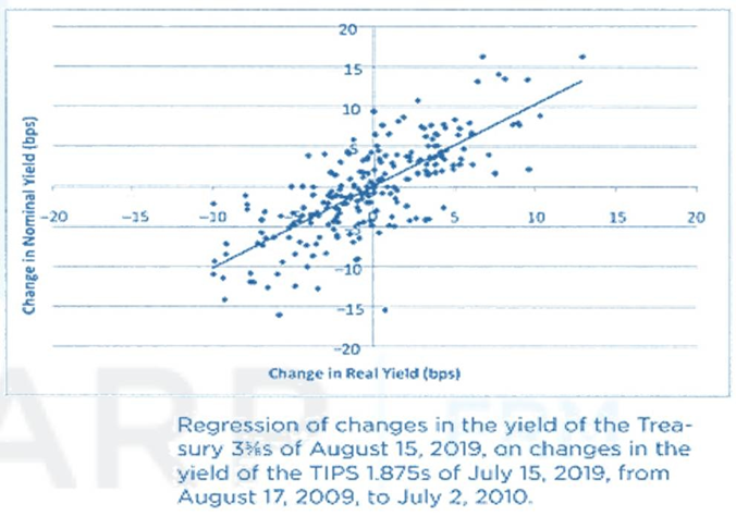
•With respect to improving on the 𝐷𝑉𝑂1 hedge, there is not much the trader can do about the  dispersion of the change in the nominal yield for a given change in the real yield. That is part  of the risk of the trade. But the trader can estimate the average change in the nominal yield for  a given change in the real yield and adjust the DV0l hedge accordingly. For example, were it to  turn out-as it will-that the nominal yield in the data changes by 1.0189 basis points per basis-  point change in the real yield, the trader could adjust the hedge such that

•As done in FRM Part 1, Least-squares estimation of 𝛼 and 𝛽 finds the estimates 𝛼^ and 𝛽^{^} that  minimize the sum of the squares of the realized error terms over the observation period. A  typical summary of the regression output is given in this table. The 𝛽^{^} reported in the table is  1.0189, which says that, over the sample period, the nominal yield increases by 1.0189 basis  points per basis-point increase in real yields. The constant term of the regression,𝛼^, is not very  different from zero, which is typically the case in regressions of changes in a yield on changes  in a comparable yield. The economic interpretation of this regularity is that a yield does not  usually trend up or down while a comparable yield is not changing.

Regression Analysis of Changes in the Yield of the 3⅝s of August 15, 2019, on the Changes in Yield of the TIPS 1⅛s of July 15, 2019, from August 17, 2009, to July 2, 2010

No. of Observations	229
R-Squared	56.3%
Standard Error	3.82
Regression Coefficients	Value	Std. Error
Constant (α)	0.0503	.2529
Change in Real Yield (β)	1.0189	.0595

•The regression-based hedge, can be written as

where

𝐹^𝑅 is the face amount of the real bond

𝐹^𝑁  is the face amount of the nominal bond

𝐷𝑉𝑂1^𝑅 is the 𝐷𝑉𝑂1 of the real bond

𝐷𝑉𝑂1^𝑁  is the 𝐷𝑉𝑂1 of the nominal bond

Least-Squares Regression Analysis

•To improve 𝐷𝑉01-neutral hedging, regression hedge can be used. This approach adjusts the  DV01 hedge based on historical volatility. A regression is carried out where the change in real  yield (∆𝑦^𝑅) is the independent variable and the change in nominal yield (∆𝑦^𝑁) is the dependent  variable. So if the average change in the nominal yield can be calculated for a given change in  the real yield, then the 𝐷𝑉01 hedge can be adjusted accordingly. So the regression hedge is the 𝐷𝑉01 hedge adjusted for the average change of nominal yields relative to real yields

•Let  ∆𝑦 ^𝑁 and  ∆𝑦 ^𝑅 be the changes in the yields of the nominal and real bonds, respectively, and assume that

Here, the changes in the real yield, the independent variable, are used to predict changes in the  nominal yield, the dependent variable. The intercept, 𝛼 , and the slope, 𝛽, need to be  estimated from the data.

As an example, suppose the parameters estimated with the data, denoted 𝛼^ and 𝛽^{^}, are 0 and 1.02 respectively. Then, if ∆𝑦^𝑅 is 5 basis points on a particular day, the predicted change if the nominal yield, written ∆𝑦^^𝑁, is ∆𝑦^^𝑁 = 𝛼^ + 𝛽^{^}∆𝑦^𝑅  = 0 + 1.02 × 5 = 5.1

The Regression Hedge

•The profit and loss (P&L) of the hedged position over a day is

•Also, beta of the hedge can be calculated as

In our example

In other words, the risk of the (TIPS) hedging portfolio, measured by 𝐷𝑉𝑂1, is 101.89% of  the risk of the underlying (nominal) position, measured by 𝐷𝑉𝑂1. Alternatively, the risk  weight of the hedge portfolio is 101.89%.

•The standard error of the regression 𝜎^ can be used to approximate the standard deviation of ∆𝑦^𝑁 − 𝛽^{^}∆𝑦^𝑅. The standard deviation of the P&L is approximately

In our example, it is

The trader would have to compare this volatility with an expected gain to decide whether or  not the risk-return profile of the trade is attractive.

•An important difficulty in using regression-based hedging in practice is that the hedger can  never be sure that the hedge coefficient, 𝛽, is constant over time. When it is stable over time, a  hedger can safely continue to use a previously estimated 𝛽 for hedging. But if it is unstable, the  hedger should re-estimate the hedge coefficient with more recent data, if available, or with data  from a past, more relevant time period.

Two-Variable Regression-Based Hedging

•To illustrate regression hedging with two independent variables, this section considers the case  of a market maker in 𝐸𝑈𝑅 interest rate swaps. The market maker has bought or received fixed  in relatively illiquid 20-year swaps from a customer and needs to hedge the resulting interest  rate exposure. Immediately paying fixed or selling 20-year swaps would sacrifice too much if  not all of the spread paid by the customer, so the market maker chooses instead to sell a  combination of 10- and 30-year swaps. A two-variable regression model to describe the  relationship between changes in 20-year swap rates and changes in 10- and 30-year swap  rates:

Using least square regression, the parameters are estimated as 𝛼^, 𝛽^{^10} and 𝛽^{^30}. The estimation  of these parameters then provides a predicted change for the 20-year swap rate:

•To derive the notional face amount of the 10- and 30-year swaps, 𝐹¹⁰ and 𝐹³⁰, respectively,  required to hedge 𝐹²⁰ face amount of the 20-year swaps, the reasoning given in the single-  variable case can be generalized. The P&L of the hedged position can be written as

Then the predicted change in the 20-year rate is substituted, retaining only the terms depending on ∆𝑦¹⁰  and ∆𝑦³⁰, to get

Finally, 𝐹¹⁰  and 𝐹³⁰  are calculated by setting the terms in brackets equal to zero, i.e., to  eliminate the dependence of predicted P&L on changes in the 10- and 30-year rates. This gives

•As in the single-variable case, this 10s-30s hedge of the 20-year can be expressed in terms of  risk weights. More specifically, the 𝐷𝑉𝑂1 risk in the 10-year part of the hedge and the 𝐷𝑉𝑂1  risk in the 30-year part of the hedge can both be expressed as a fraction of the 𝐷𝑉𝑂1 risk of  the 20-year. Mathematically, these risk weights can be found as

•Results for the regression analysis of changes in the 20-  year 𝐸𝑈𝑅 swap rate on changes in the 10- and 30-year

𝐸𝑈𝑅 swap rates from July 2, 2001, to July 3, 2006 are

given in this table. Applying the risk-weight  interpretation of the regression coefficients it is  calculated that 22.21% of the 𝐷𝑉01 of the 20-year  swap should be hedged with a 10-year swap and  77.65% with a 30-year swap. The sum of these weights,  99.86%, happens to be very close to one, meaning that  the 𝐷𝑉01 of the regression hedge very nearly matches the 𝐷𝑉01 of the 20-year swap.

Regression Analysis of Changes in the Yield of the 20-Year EUR Swap Rate on Changes in the 10- and 30-Year EUR Swap Rates from July 2, 2001, to July 3, 2006

No. of Observations	1281
R-Squared	99.8%
Standard Error	0.14
Regression Coefficients	Value	Std. Error
Constant (α)	-0.0014	0.0040
Change in 10-Year Swap Rate (β10)	0.2221	0.0034
Change in 30-Year Swap Rate (β30)	0.7765	0.0037

Level Versus Change Regressions

•When estimating regression-based hedges, some practitioners regress changes in yields on  changes in yields, as in the previous sections, while others prefer to regress yields on yields.  Mathematically, in the single-variable case, the level-on-level regression with dependent variable  y and independent variable x is

𝑦_𝑡 = 𝛼 + 𝛽𝑥_𝑡 + c_𝑡

while the change-on-change regression is

𝑦_𝑡 − 𝑦_𝑡−1 = ∆𝑦_𝑡 = 𝛽∆𝑥_𝑡 + ∆c_𝑡

•By theory that is beyond the scope of the FRM curriculum, it is known that if the error terms  c_𝑡 are independently and identically distributed random variables with mean zero and are  uncorrelated with the independent variable, then so are the ∆c_𝑡, and least squares on either of  the above will result in coefficient estimators that are unbiased, consistent, and efficient, i.e., of  minimum variance, in the class of linear estimators. If the error terms of either specification  are not independent of each other, however, then the least-squares coefficients of that  specification are not necessarily efficient, but retain their unbiasedness and consistency. There is  a more sensible way to model the relationship between two bond yields than either of the above by assuming the error dynamics c_𝑡 = 𝜌c_𝑡−1 + 𝑣_𝑡 for some constant 𝜌 < 1.

Principal Components Analysis

•Regression analysis tries to explain the changes in the yield of one bond relative to changes in the yields  of a small number of other bonds. It is often useful, however, to have a single, empirical description of  the behaviour of the term structure that can be applied across all bonds. Principal Components (PCs)  provide such an empirical description.

•To fix ideas, consider the set of swap rates from 1 to 30 years at annual maturities. One way to describe  the time series fluctuations of these rates is through the variances of the rates and their pairwise  covariances or correlations. Another way to describe the data, however, is to create 30 interest rate factors  or components, where each factor describes a change in each of the 30 rates. So, for example, one factor  might be a simultaneous change of 5 basis points in the 1-year rate, 4.9 basis points in the 2-year rate,

8.basis points in the 3-year rate, etc. Principal Components Analysis (𝑃𝐶𝐴) sets up these 30 such  factors with the following properties:

1.The sum of the variances of the PCs equals the sum of the variances of the individual rates. In this  sense the PCs capture the volatility of this set of interest rates.

2.The PCs are uncorrelated with each other. While changes in the individual rates are, of course,  highly correlated with each other, the PCs are constructed so that they are uncorrelated.

3.Subject to these two properties or constraints, each PC is chosen to have the maximum possible  variance given all earlier PCs. In other words, the first PC explains the largest fraction of the  sum of the variances of the rates; the second PC explains the next largest fraction, etc.

•𝑃𝐶s of rates are particularly useful because of an empirical regularity: the sum of the variances  of the first three 𝑃𝐶s is usually quite close to the sum of variances of all the rates. Hence,  rather than describing movements in the term structure by describing the variance of each rate  and all pairs of correlation, one can simply describe the structure and volatility of each of only  three PCs. The results of PCA provide a great deal of comfort to hedgers: while in theory  many factors (and, therefore, securities) might be required to hedge the interest rate risk of a  particular portfolio, in practice, three factors cover the vast majority of the risk.

•𝑃𝐶𝐴 is useful for constructing empirically based hedges for large portfolios; it is impractical to  perform and assess individual regressions for every security in a large portfolio.