Counterparty Risk And Credit Exposure

Microsoft PowerPoint – CR 12 – Credit Exposure and Funding

• A defining characteristic of counterparty risk arises from the asymmetry of potential losses with respect to value of the underlying transactions. The effective value of the contracts (including collateral) can be positive (in an institution’s favor) or negative (against them) :
  • Positive Value When a counterparty defaults, they will be unable to make future commitments and hence an institution will have a claim on the positive value at the time of the default. The loss given default will be equal to the amount of this value minus any recovery value.
  • Negative Value In this case, an institution owes its counterparty and is legally obliged to settle this amount. An institution does not gain or lose from their counterparty’s default in this case.
• The above feature-an institution loses if the value is positive and does not gain if it is negative- is a defining characteristic of counterparty risk. We can define exposure simply as: Exposure = Max(Value,0).

Bilateral Exposure

• A key feature of counterparty risk is that it is bilateral as both parties to a transaction can default and therefore both can experience losses. For completeness, one must consider losses arising from both defaults. From an institution’s point of view, their own default will cause a loss to any counterparty they are in debt to. This can be defined in terms of negative exposure, which by symmetry is Negative Exposure = Min(Value, 0).

Exposure And A Short Option Position

Microsoft PowerPoint – CR 12 – Credit Exposure and Funding

• The asymmetric risk profile created by counterparty risk can be likened to a short option position. We can make two obvious conclusions about the quantification of exposure:
  • Since exposure is similar to an option payoff, a key aspect will be volatility (of the value of the relevant contracts and collateral).
  • Options are relatively complex to price (compared with the underlying instruments at least). Hence, to quantify credit exposure even for a simple instrument may be quite complex.
• By symmetry, an institution has long optionality from their own default. We note that this is not relevant from a risk management or regulatory point of view but may be relevant for pricing.

Comparison to VaR

• The characterization of credit exposure is similar to the characterization of VaR, but with some additional complexities with respect to :
  • Time Horizon
  • Risk Mitigants
  • Application

Comparison to VaR – Time Horizon

• Unlike VaR, exposure needs to be defined over multiple time horizons (often far in the future) so as to understand fully the impact of time and specifics of the underlying contracts. There are two important implications of this.
  • Firstly, “ageing” of transactions must be considered. Credit exposure must consider all future contractual payments and changes such as cashflows, termination events, exercise decisions and collateral postings. Such effects may also create path dependency where the exposure at one date depends on an event defined at a previous date. In VaR models, such aspects can be neglected due to the short time horizon used.
  • The trend (also known as drift) of market variables, along with their underlying volatility and co-dependence structure, is relevant for credit exposure. In VaR the drift can be ignored, again since the relevant time horizon is short.

Comparison to VaR – Risk Mitigants

• Exposure is typically reduced by risk mitigants such as netting and collateral, and the impact of these mitigants must be considered in order to properly estimate future exposure. In some cases, such as applying the correct netting rules, this requires knowledge of the relevant contractual agreements and their legal interpretation in the jurisdiction in question. In the case of future collateral amounts, another degree of subjectivity is created since there is no certainty over the type of collateral and precise time that it would be received. Other contractual features of transactions, such as termination agreements, may also create subjectivity and all such elements must be modelled, introducing another layer of complexity and uncertainty.

Comparison to VaR – Application

• VaR is a risk management approach. Exposure must be defined for both risk management and pricing (i.e., CVA). This creates additional complexity in quantifying exposure and may lead to two completely different sets of calculations, one to define exposure for risk management purposes and another for pricing (or valuation) purposes.

Future Exposure

• Although the current (and past) exposure is known with certainty, the future exposure is defined probabilistically by what may happen in the future in terms of market movements and contractual features of transactions, both of which are uncertain. Hence, in understanding future exposure we should not only define the level of the exposure, but also its underlying uncertainty.

Source: Figure 12-2, 2019 Financial Risk Manager Part II, Credit Risk Measurement and Management, 7^th Edition, by GARP

Metrics For Exposure

The total number of relevant transactions, netted appropriately and including any relevant collateral amounts is referred to as the “netting set” in all the definitions.

EXPECTED FUTURE VALUE or EXPECTED MtM

• The component represents the forward or expected value of the netting set at some point in the future. For counterparty risk, the expected value can be an important component due the longer time horizon involved but for market risk VaR assessment, it is not significant because of a shorter time horizon being used. Expected future value (EFV) represents the expected (average) of the future value calculated with some probability. EFV may vary significantly from current value due to the following
  • Cash flow differential
  • Forwards Rates
  • Asymmetric collateral agreements

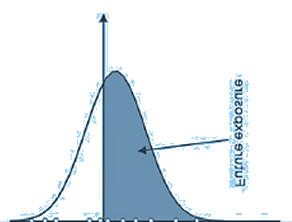
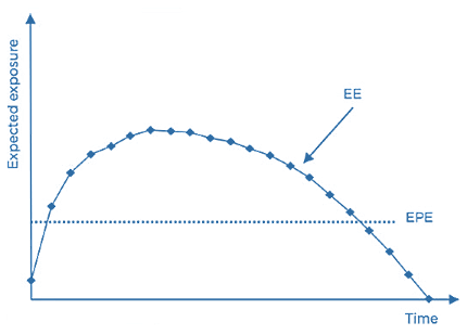
Expected Exposure

• This is the average of all exposure values. Note that only positive values (the grey area) give rise to exposure and other value have a zero contribution (although they contribute in terms of their probability). This means that the expected exposure will be more than or above the EFV (or Expected MtM) as EFV considers both positive as well as negative MtM values.

Source: Figure 12-4, 2019 Financial Risk Manager Part II, Credit Risk Measurement and Management, 7^th Edition, by GARP

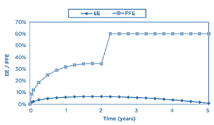
Potential Future Exposure

• Potential Future Exposure (PFE) is the maximum expected credit exposure over a specified period of time calculated at some level of confidence. For example, the PFE at a confidence level of 99% will define an exposure that would be exceeded with a probability of no more than 1% (one hundred percent minus the confidence level). PFE is a similar metric to VaR with two differences. First, while VaR is an exposure due to a market loss, PFE is a credit exposure due to a gain. Second, while VaR typically refers to a short-term horizon (for example, one or 10 days), PFE often looks years into the future.

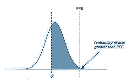
Source: Figure 12-3, 2019 Financial Risk Manager Part II, Credit Risk Measurement and Management, 7^th Edition, by GARP

Maximum PFE

• Maximum of peak PFE simply represents the highest PFE value over a given time interval, thus, representing the worst-case exposure over the entire interval. Maximum PFE is sometimes used as a metric in credit limits management.

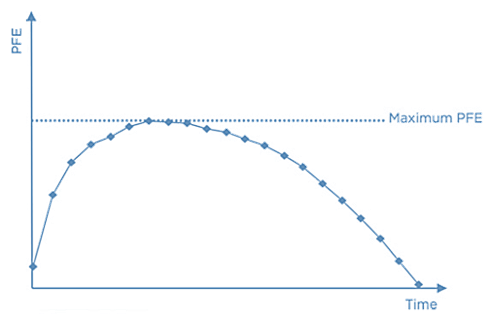
Source: Figure 12-5, 2019 Financial Risk Manager Part II, Credit Risk Measurement and Management, 7^th Edition, by GARP

Expected Positive Exposure

• Expected positive exposure (EPE) is defined as the average exposure across all time horizons. It can therefore be represented as the weighted average of the EE across time. The single EPE number is often called a “loan equivalent” , as the average amount effectively lent to the counterparty in questions. EPE has a strong theoretical basis for assessing regulatory capital and qualifying xVA.

Source: Figure 12-6, 2019 Financial Risk Manager Part II, Credit Risk Measurement and Management, 7^th Edition, by GARP

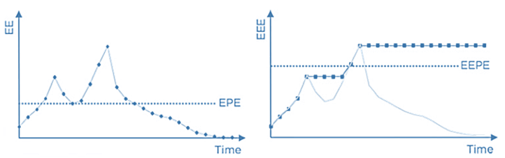
Negative Exposure

• Exposure is represented by positive future values. Conversely, we may define negative exposure as being represented by negative future values. This will obviously represent the exposure from a counterparty’s point of view. We can therefore define measures such as negative expected exposure (NEE) and expected negative exposure (ENE), which are the precise opposites of EE and EPE.

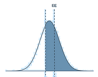
Effective Expected Positive Exposure

• For these reasons, EEPE was introduced for regulatory capital purposes (BCBS, 2005). It is the average of the effective EE (EEE), which is simply a non-decreasing version of the EE profile. These terms are shown in comparison with EE and EPE. EEPE assumes that any reduction in the EE profile is a result of a maturing transaction that will be replaced.

Source: Figure 12-7, 2019 Financial Risk Manager Part II, Credit Risk Measurement and Management, 7^th Edition, by GARP

Factors Driving Credit Exposure Profile

Future Uncertainty

• The first and most obvious driving factor in exposure is future uncertainty. Forward contracts such as forward rate agreements (FRAs) and FX forwards are usually characterized by having just the exchange of two cashflows (often netted into a single payment) at a single date, which is the maturity of the contract. If we assume that the returns of the underlying market variable (e.g. FX) are independently identically distributed, then it can be shown that such a profile will follow a “square root of time” rule, meaning that it will be proportional to the square root of the time (t)

\(\text{Exposure} \propto \sqrt{t}\)

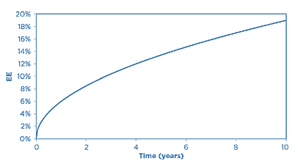
Source: Figure 12-8, 2019 Financial Risk Manager Part II, Credit Risk Measurement and Management, 7^th Edition, by GARP

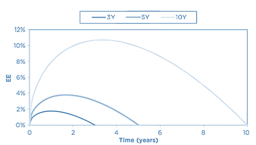
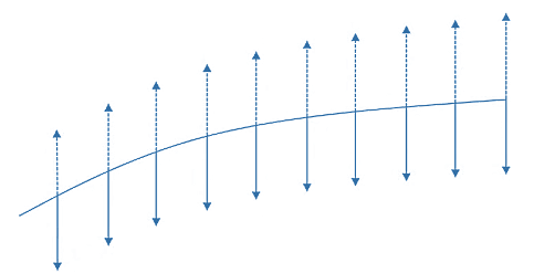
Periodic Cash Flows

• Many OTC derivatives include the periodic payment of cashflows, which has the impact of reversing the effect of future uncertainty. The most obvious and common example here is an interest rate swap, which is characterised by a peaked shape. The shape arises from the balance between future uncertainties over payments, combined with the roll-off of fixed against floating payments over time. This can be represented approximately as

\(\text{Exposure} \propto (T – t)\sqrt{t}\)

where T represents the maturity of the transaction in question.

• The above function is initially increasing due to the \(\sqrt{t}\) term, but then decreases to zero as a result of the (T – t) component, which is an approximate representation of the remaining maturity of the transaction at a future time t. It can be shown that the maximum of the above function occurs at T/3, i.e. the maximum exposure occurs at one-third of the lifetime.

• A swap with a longer maturity has much more risk due to both the increased lifetime and the greater number of payments due to be exchanged.

Source: Figure 12-9, 2019 Financial Risk Manager Part II, Credit Risk Measurement and Management, 7^th Edition, by GARP

• An exposure role can be substantially altered due to the more specific nature of the cashflows in a transaction. Transactions such as basis swaps, where the payments are made more frequently than they are received (or vice versa) will then have more (less) risk than the equivalent equal payment swap.

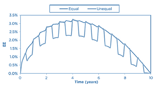
Source: Figure 12-10, 2019 Financial Risk Manager Part II, Credit Risk Measurement and Management, 7^th Edition, by GARP

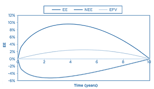
• In a “payer swap”, fixed cashflows are paid periodically at a fixed rate whereas floating cashflows are received. The value of future floating cashflows is not known until the fixing date, although at inception their (risk-neutral) expected value will be equal to that of the fixed cashflows. The value of the projected floating cashflows depends on the shape of the underlying yield curve. In the case of a typical upwards-sloping yield curve, the initial floating cashflows will be expected to be smaller than the fixed rate paid, whilst later in the swap the trend is expected to reverse.

Source: Figure 12-13, 2019 Financial Risk Manager Part II, Credit Risk Measurement and Management, 7^th Edition, by GARP

• The net result of the previous effect is that the EE of the payer swap is higher due to the expectation to pay net cashflows (the fixed rate against the lower floating rate) in the first periods of the swap, and receive net cashflows later in the lifetime. The NEE is correspondingly less negative. Another way to state this is that the EFV of the swap is positive.
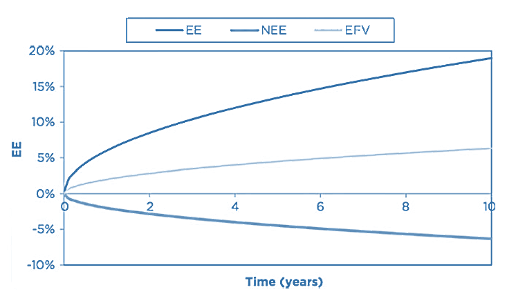
• For an opposite “receiver” swap, this effect would be reversed with the EE being lower, NEE more negative and the sign of the EFV reversed.

Source: Figure 12-14, 2019 Financial Risk Manager Part II, Credit Risk Measurement and Management, 7^th Edition, by GARP

• The previous effect can be even more dramatic in cross-currency swaps where a high interest- rate currency is paid against one with lower interest rates. (as was the case, for example, with widely traded dollar versus yen swaps for many years before the dramatic US interest rate cuts of 2008/09).

Source: Figure 12-15, 2019 Financial Risk Manager Part II, Credit Risk Measurement and Management, 7^th Edition, by GARP

Combination of Profiles

• Some products have an exposure that is driven by a combination of two or more underlying risk factors. An obvious example is a cross-currency swap, which is essentially a combination of an interest rate swap and an FX forward transaction. This would therefore be represented by a combination of the profiles of those two instruments.
• Cross-currency swap exposures can be considerable due to the high FX volatility driving the risk, coupled with the long maturities and final exchanges of notional. The contribution of the interest rate swap is typically smaller, as shown. We note also that the correlation between the two interest rates and the FX rate is an important driver of the exposure. A relatively low correlation, as often seen in practice, increases the cross-currency exposure.

Source: Figure 12-17, 2019 Financial Risk Manager Part II, Credit Risk Measurement and Management, 7^th Edition, by GARP

• The longer maturity swaps have slightly more risk due to the greater number of interest rate payments on the swap.

Source: Figure 12-17, 2019 Financial Risk Manager Part II, Credit Risk Measurement and Management, 7^th Edition, by GARP

Optionality

• The impact of exercise decisions creates some complexities in exposure profiles, since after the exercise date(s) the underlying transaction will have a certain probability of being “alive” or not. This is particularly important in the case of physical settlement.
• This figure shows the exposure for a European- style interest rate swaption that is swap-settled (physical delivery) rather than cash-settled. The underlying swap has different payment frequencies also. It is compared with the equivalent forward starting swap. Before the exercise point, the swaption must always have a greater exposure than the forward starting swap, but thereafter this trend will reverse, since there will be scenarios where the forward starting swap has positive value but the swaption would not have been exercised.

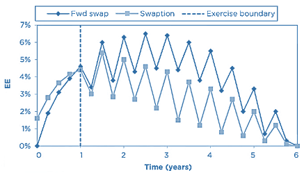
Source: Figure 12-18, 2019 Financial Risk Manager Part II, Credit Risk Measurement and Management, 7^th Edition, by GARP

Credit Derivatives

• Credit derivatives represent a big problem for counterparty risk assessment due to wrong- way risk. Even without this as a consideration, exposure profiles of credit derivatives are hard to characterize due to the discrete payoffs of the instruments.

Source: Figure 12-20, 2019 Financial Risk Manager Part II, Credit Risk Measurement and Management, 7^th Edition, by GARP

• This figure shows the exposure profile of a single- name CDS. While the EE shows a typical swap-like profile, the PFE has a jump due to the default of the reference entity. it means that PFE may or may not represent the actual credit event occurring and is sensitive to the confidence level used. Using a measure such as expected shortfall15 partially solves this problem. This effect will also not be apparent for CDS indices due to the large number of reference credits where single defaults have a less significant impact.

Impact of Netting On Exposure

• This figure illustrates the impact of netting on exposure with exactly opposite transactions. When there is no legal agreement to allow netting, then exposures must be considered additive. This means that the positions do not offset one another. With netting permitted (and enforceable), one can add values at the netting set level before calculating the exposure and therefore the profiles shown give a zero exposure at all points in the future. This means that two opposite transactions (as shown in the example) will give a zero exposure with netting.

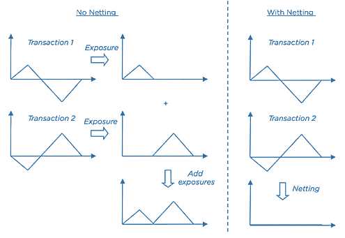
Source: Figure 12-21, 2019 Financial Risk Manager Part II, Credit Risk Measurement and Management, 7^th Edition, by GARP

Netting And The Impact Of Correlation

• Netting is essentially a diversification effect. When considering the netting benefit of two or more transactions, the most obvious consideration is the correlation between the future values (and therefore exposures also). A high positive correlation between two transactions means that future values are likely to be of the same sign. This means that the netting benefit will be small or even zero. For example, in this table, the two sets of values create very little netting benefit, and netting is beneficial in only one out of the five scenarios.

Scenario	Future value		Total Exposure		Netting Benefit
	Trade 1	Trade 2	No Netting	Netting
Scenario 1	25	15	40	40	0
Scenario 2	15	5	20	20	0
Scenario 3	5	-5	5	0	5
Scenario 4	-5	-15	0	0	0
Scenario 5	-15	-25	0	0	0
EE			13	12	1

• On the other hand, negative correlations are clearly more helpful as future values are much more likely to have opposite signs and hence the netting benefit will be stronger. This is illustrated in the following table, where netting is beneficial in four out of the five scenarios.

Scenario	Future value		Total Exposure		Netting Benefit
	Trade 1	Trade 2	No Netting	Netting
Scenario 1	25	-15	25	10	15
Scenario 2	15	-5	15	10	5
Scenario 3	5	5	10	10	0
Scenario 4	-5	15	15	10	5
Scenario 5	-15	25	25	10	15
EE			18	10	8

The formula for the “netting factor” with respect to exposure under the assumption that future values follow a multivariate normal distribution, is given by :

\(NF = \frac{\sqrt{n + n(n – 1) \bar{\rho}}}{n}\)

where

n is the number of exposures,

\(bar{\rho}\) is the average correlation

The netting factor represents the ratio of net to gross exposure and will be +100% if there is no netting benefit (ρ ̅ = 1) and 0% if the netting benefit is maximum. The netting benefit improves (i.e., NF decreases) with a larger value of n and a lower value of ρ ̅. If ρ ̅=0, the NF becomes 1/√n . This means, for example, that two independent transactions with zero mean and equal volatility have a netted exposure reduced to 71% (1/√2) of their exposure without netting. For five exposures, the netting factor decreases to 45% (1/√5).

Netting and Relative MtM

• Netting benefit depends not only on the correlation of future values but also on their relative offset. Negative future value will create netting benefit irrespective of the structural correlation between transactions.

Impact Of Collateral On Exposure

• A simple example of the impact of collateral on exposure is given in this table, assuming a two-way collateral agreement. In scenarios 1 to 3, the exposure is reduced significantly, since collateral is held. The exposure is not perfectly collateralized, which may be the case in practice due to factors such as a sudden increase in MtM, or contractual aspects such as thresholds and minimum transfer amounts. In scenario 4, the value of the portfolio is negative and collateral must therefore be posted but this does not increase the exposure. Finally, in scenario 5, the posting of collateral creates exposure. In comparison with the benefits shown in the other scenarios, this is not a particularly significant effect, but it is important to note that collateral can increase as well as reduce exposure.

Scenario	Future value		Exposure		Benefit
	Portfolio	Collateral	No Collateral	With Collateral
Scenario 1	25	23	25	2	23
Scenario 2	15	12	15	3	12
Scenario 3	5	3	5	2	3
Scenario 4	-5	2	0	0	0
Scenario 5	-15	-18	0	3	-3
EE			9	2	-7

• To the extent that collateral is not a perfect form of risk mitigation, there are three considerations:
  • There is a granularity effect because it is not always possible to ask for all of the collateral required, due to parameters such as thresholds and minimum transfer amounts. This can sometimes lead to a beneficial overcollateralization  where the collateral amount is for a short period greater than the exposure. Note that this must also consider the impact of collateral that a party must themselves post.
  • There is a delay in receiving collateral that involves many aspects such as the operational components of requesting and receiving collateral to the possibility of collateral disputes. These aspects are included in the assessment of the MPR.
  • We must consider a potential variation in the value of the collateral itself (if it is not cash in the currency in which the exposure is assessed).

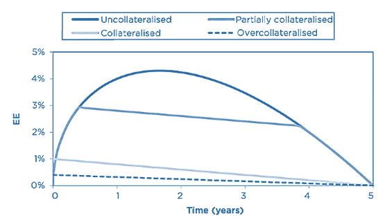
DIFFERENT LEVELS OF COLLATERALIZATION

• Partially collateralized –  Here, the presence of contractual aspects such as thresholds means that the reduction of exposure is imperfect. A threshold can be seen as approximately capping the exposure.
• Collateralized –  In the collateralized case, we assume aspects such as thresholds are zero and therefore the exposure is reduced significantly. However, the MPR still leads to a reasonably material value.
• Overcollateralized –  In this case, we assume there is initial margin and therefore the exposure is reduced further compared to the above case (and potentially to zero if the initial margin is large enough).

This figure shows the qualitative impact for the three cases

REMARGIN PERIOD

• The remargin period, also known as the margin call frequency, is the period from which a collateral call takes place to when collateral is actually delivered. It is a period of extreme exposure to the counterparty seeking collateral.
• To calculate remargin period, the following effects must be considered as they may slow down the collateral process:
  • Valuation/margin call – This is the time taken to calculate current exposure to the counterparty and the market value of the collateral, determining if a valid call can be made and finally making that call. This should include the time delay due to the contractual period between margin calls
  • Receiving collateral – The time gap between a counterparty receiving a collateral request) to the point at which they release collateral. The possibility of a dispute  should be incorporated here.
  • Settlement – This represents the time it takes to sell the collateral for cash. The type of security being settled determines the time necessary. Cash collateral may settle on an intraday basis whereas other securities will take longer. For example, government and corporate bonds may be subject to 1-day and 3-day settlement periods, respectively.
  • Grace period – The amount of time afforded to the counterparty obligated to deliver the collateral in the event that the collateral is not received by the requesting counterparty after the call. If the collateral is not received even after the grace period is over, the counterparty would be deemed to be in default. This is sometimes known as the cure period.
  • Liquidation/closeout and re-hedge – This is the time needed to liquidate the collateral, close out, and re-hedge positions.
• Under Basel II rules the minimum margin period of risk which must be assumed for OTC derivatives is 10 (business) days assuming collateral may be called for on a daily basis. OTC derivatives and repo transactions are considered separately since they are governed by different documentation. Collateralization in repo markets is generally tighter and the minimum period assumed is therefore lower partly due to the more complex nature of OTC derivatives, which makes valuation more complex.
• Other parameters which determine the reduction of credit exposure due to collateral are :
  • Threshold: An exposure level below which collateral is not called. It represents an amount of uncollateralized exposure.
  • Minimum Transfer Amount: The minimum quantity or block in which collateral may be transferred. Quantities below this amount represent uncollateralized exposure as well.
  • Initial Margin: The amount posted initially which is independent of any collateralization.
  • Rounding: The process by which a collateral call amount will be rounded off to a certain value.

Funding Costs And Benefits (Optional)

• The concept of funding costs and benefits has clear similarities with the definition of exposure. A positive value is at risk when a counterparty defaults, but is also the amount that has to be funded when the counterparty does not. A negative exposure is associated with a funding benefit. However, there are some distinct differences that must be considered:
  • Close-out – The consideration of potential close-out adjustments is relevant only in the definition of credit exposure in a default scenario and does not apply when considering funding aspects that should be based on the MTM.
  • Margin period of risk – The MPR is a concept that is defined assuming the default of the counterparty and is relevant for credit exposure. In assessing the equivalent delay in receiving collateral against a derivatives portfolio, the normal collateral posting frequency (which is likely much shorter) should be assumed. This is one reason why the FVA of a collateralized derivative may be considered to be zero, even though the equivalent CVA is not.
  • Netting – Close-out netting is a concept that applies in a default scenario and hence credit exposure is defined at the netting set level (which may correspond or be a subset of the counterparty level). On the other hand, funding applies at the overall portfolio level since MTM for different transactions is additive and collateral received from one counterparty may be posted to another.
  • Segregation – Segregation has different impacts on credit exposure and funding.

Despite the above differences, credit, debt and funding value adjustments (CVA, DVA and FVA) have many similarities and should most obviously be quantified using shared methodologies.