Pricing Counterparty Risk – Motivation

• Accurate pricing of counterparty risk involves attaching a value to the risk of all outstanding positions with a given counterparty. This is important for the following reasons:
  • It helps in the reporting of accurate profit and loss information.
  • It provides incentives to trading desks and businesses to trade appropriately.
  • The reserves generated absorb potential losses in the event of the counterparty’s default.
  • Pricing counterparty risk also accounts for risk mitigants.
• Pricing credit risk for an instrument with one-sided payments is relatively straightforward as we simply need to account for default when discounting the cashflows and add the value of any payments made in the event of a default. However, many derivatives instruments have fixed, floating, or contingent cashflows or payments that are made in both directions. This bilateral nature determines the credit exposure and makes the quantification more difficult.

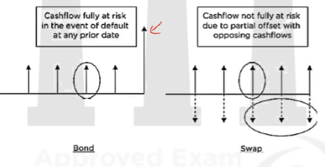
• For example, this figure compares a bond to a similar swap transaction. In the bond case, a portion of a given cashflow is fully at risk in case of default, whereas in the swap, only part of the cashflow will be at risk due to partial cancellation with opposing cashflows. The risk on the swap is smaller due to this effect. However, the fraction of the swap cashflows that are indeed at risk is hard to determine as this depends on many factors such as yield curve shape, forward rates, and volatilities.

Credit Value Adjustment (CVA) – Description

• The credit value adjustment (CVA) represents the market value or price of counterparty credit risk.
• CVA was originally introduced as an adjustment to the risk-free value of a derivative to account for potential default using the following relationship:
  Risky value = Risk-free value – CVA
• The obvious proxy for the risk-free value is OIS discounting. Historically, this relationship was seen as a “credit charge” for pricing and a “reserve” or “provision” for financial reporting purposes. There is a hidden complexity in the above relationship, which is that it is not naturally additive across transactions. Due to risk mitigants such as netting and collateral, CVA must be calculated for all transactions covered by these risk mitigants. The impact of collateral will also be non-additive.
• In practice, as well as in accounting standards, it’s a bilateral calculation, i.e., it prices the credit risk faced by both the bank and the counterparty.

Credit Value Adjustment (CVA) – Formula

• The standard formula for computation of CVA is:

\(CVA = -LGD \sum_{i=1}^{m} EE(t_i) \times PD(t_{i-1}, t_i)\)

where

• LGD (Loss given default) is the percentage amount of the exposure expected to be lost if the counterparty defaults. LGD = 100% – RR (Recovery Rate).
• EE (Expected Exposure) is the discounted expected exposure for the relevant dates in the future given by \(t_i\) for i=1,2,…m. Although discount factors could be represented separately, it is usually most convenient to apply (risk-free) discounting during the computation of the EE.
• PD (Default Probability) represents the marginal default probability in the interval between time \(t_{i-1}\) and \(t_i\).
• There is a minus sign to signify that CVA is a loss. This convention was not always followed in the past, but is relevant since CVA in general can have both positive and negative impacts.
• An advantage of computing CVA using this formula is that default enters the expression via default probability only. This means that, while one may require a simulation framework in order to compute CVA, it is not necessary to simulate default events, only the exposure (EE). This saves on computation time by avoiding the need to simulate relatively rare defaults.
• The formula assumes that the credit exposure and default probability are independent, i.e., there is no wrong-way risk. This further simplifies the calculations

CVA as a Spread

• Instead of being computed as stand-alone value, CVA can also be expressed as a spread (per annum charge).
• A simple calculation would involve dividing the CVA by the risky annuity value for the maturity in question. There is also a quicker way if it is assumed that the EE is constant over time and equal to its average value (EPE). This yields the following approximation based on EPE:

CVA ~ -EPE X spread …(C)

where

EPE is the average exposure across all time horizons, and hence, can be represented as the weighted average of the EE across time.

CVA is expressed in the same units as the credit spread

• This approximate formula tends to be more accurate for swap-like profiles, where the symmetry of the profile helps, but is less accurate for monotonically increasing profiles. It is also more accurate where the default probabilities are relatively constant.

Risk Neutrality

• In general, is computed with risk-neutral (market-implied) parameters. This approach defines the price with respect to hedging instruments and supports the exit price concept required by accounting standards. But certain parameters cannot be risk-neutral, since they are not observed in the market (e.g. correlations), or may require interpolation or extrapolation assumptions (e.g. volatilities). Risk-neutral parameters such as volatilities may generally be higher than their real-world equivalents (e.g. historical estimates).
• The use of risk-neutral default probabilities may be questioned for a number of reasons:
  • Risk-neutral default probabilities are significantly higher than their real-world equivalents.
  • Counterparties do not have liquid single-name credit default swaps referencing them.
  • The business model of banks is generally to “warehouse” credit risk, and they are therefore only exposed to real-world default risk.

Credit Spread Impact

• The impact of increasing the credit spread of the counterparty is expressed in the given table The increase in credit spread clearly increases the CVA, but this effect is not linear since default probabilities are bounded by 100%. Another way to understand this is that the “jump to default” risk of this swap is zero, since it has a current value of zero and so an immediate default of the counterparty will (theoretically) not cause any loss. As the credit quality of the counterparty deteriorates, the CVA will obviously decrease (become more negative) but at some point, when the counterparty is close to default, the CVA will increase again.

Spread (bps)	CVA
150	-1,074
300	-1,999
600	-3,471
1,200	-5,308
2,400	-6,506
4,800	-6,108
9,600	-4,873
Default	0

• The impact of curve shape on the is expressed in the given table. For the five-year swap, even though the spread at the maturity is fixed, there are quite different results for the different curve shapes. Indeed, going from an upwards-sloping to a flat curve changes the by around 10%. For the ten-year swap, we are extrapolating the known five-year spread and the differences are even more extreme: the upwards-sloping curve gives a more than double the downwards-sloping curve. Hence the shape of the credit curve as being an important part of the mapping process.

	Five-year	Ten-year
Upwards-sloping	-2,179	-6,526
Flat	-1,999	-4,820
Downwards-sloping	-1,690	-2,691

Recovery Impact

• Settled recovery defines the (expected) LGD at the time of default whereas the actual recovery defines the (expected) LGD that will actually be experienced. While they are different conceptually, if a derivatives claim is of the same seniority as that referenced in the CDS (as is typically the case), then we should assume that \(LGD_{settled} = LGD_{actual}\).
• The impact of changing settled and actual LGDs on the CVA is expressed in the given table. Increasing LGD reduces the risk-neutral default probability but increases the loss in the event of default. The net impact is reducing the CVA by a small amount. Using different assumptions for settled and actual LGDs will change the CVA more significantly. For example, assuming a 90% settled LGD and a lower 60% actual LGD (similar to the values experienced in the Lehman Brothers bankruptcy) gives a much higher (less negative) CVA.

LGD (settled/final)	CVA
80% both	-2,072
60% both	-1,999
40% both	-1,862
90%/60%	-1,398

Netting And Incremental CVA

• When there is a netting agreement then the impact will reduce the CVA and cannot increase it. Therefore, for a netting set (a group of transactions with a given counterparty under the same netting agreement):

\(CVA_{NS} \geq \sum_{i=1}^{n} CVA_i\)

where \(CVA_{NS}\) is the total CVA of all transactions under the NS netting agreement and \(CVA_{i}\) is the stand-alone for transaction i.

• This reduction effect ( becoming less negative) can be significant and the question is how to allocate the netting benefits to each individual transaction. The most obvious way to do this is to use the concept of incremental . Here the of a transaction is calculated based on the incremental effect this transaction has on the netting set:

\(CVA_i^{incremental} = CVA_{NS+i} – CVA_{NS}\)

where \(CVA_{NS+i} = CVA\) including trade i in the netting set

• This formula ensures that the CVA of a specified transaction is given by its contribution to the overall CVA at the time it is executed. Hence, it makes sense when the CVA needs to be charged to individual salespeople, traders or businesses. The CVA depends on the order in which transactions are executed but does not change due to subsequent transactions. An xVA desk charging this amount will directly offset the instantaneous impact on their total MtM from the change in CVA from the new transaction.
• The formula for incremental can be derived as:

\(CVA_i^{incremental} = -LGD \sum_{i=1}^{m} EE_i^{incremental}(t_i) \times PD(t_{i-1}, t_i)\)

• Incremental FE can be negative, due to beneficial netting effects, which will lead to a being positive and, in such a case, it would be a benefit and not a cost.
• Due to the properties of EE and netting, the incremental CVA in the presence of netting will never be lower (more negative) than the stand-alone CVA without netting. The practical result of this is that a party with existing transactions under a netting agreement will be likely to offer conditions that are more favorable with respect to a new transaction.
• Also, the value of incremental CVA will approach standalone CVA, if the transaction becomes larger and larger, and the benefit will be reduced.

Incremental CVA – Example (Optional Slide)

• The under the assumption of five different existing transactions with the counterparty, for a seven-year interest rate swap, is expressed in the following table :
• The following observations can be made:
  • The incremental CVA is never lower (more negative) than stand-alone CVA, since netting cannot increase exposure.
  • The incremental CVA is only slightly less negative for a very similar existing transaction (five-year payer EUR swap). This follows from the high positive correlation between the two transactions. The swaption also leads to only a small reduction due to the directionality.
  • The incremental CVA is increased (less negative) significantly for the cross-currency swap and the receiver swap. In the latter case, we may have expected a positive CVA, which is not the case (but this reversal effect is seen for DVA later).

Marginal CVA

• Marginal CVA may be useful to break down a CVA for any number of netted transactions into transaction-level contributions that sum to the total CVA. It can be used to analyze which of the trades affect the counterparty’s CVA the most . It provides an ex-post view of the trades.
• It can be calculated by simply including the marginal EE in the CVA formula (B).
• While marginal CVA might not be used for pricing new transactions (due to the problem that marginal CVA changes when new transactions are executed, implying MtM adjustment to trading books), it may be required for pricing transactions executed at the same time (perhaps due to being part of the same deal) with a given counterparty.
• Alternatively, marginal CVA is the appropriate way to allocate a CVA to transaction level contributions at a given time. This may be useful for reporting purposes or to give an idea of transactions that could be usefully restructured, novated or unwound.

Marginal CVA – Example

• The following table shows the incremental and marginal corresponding to the interest rate swap (Payer IRS 7Y) and the cross-currency swap (xCCY USDJPY) with exposures assuming a credit curve at 300 bps flat.

	Incremental (IRS first)	Incremental (CCS first)	Marginal
IRS	-0.4838	-0.2587	-0.3318
CCS	-0.1990	-0.4241	-0.3510
Total	-0.6828	-0.6828	-0.6828

• We see the effect that the first transaction is charged for the majority of the CVA, as seen before, whilst the marginal CVA charges are more balanced.

Marginal Versus Incremental CVA

Marginal CVA	Incremental CVA
DOES NOT DEPEND on the sequence of the trades	DEPENDS on the sequence of the trades
With the introduction of a new transaction, the marginal CVAs for previous transactions CHANGE	With the introduction of a new transaction, the incremental CVAs for previous transactions DO NOT change
NOT APPROPRIATE for pricing new transactions	APPROPRIATE for pricing new transactions. Incremental CVA makes more sense when charged to businesses, traders, etc.
Represents CONTRIBUTION of transaction to total CVA (analogous to Component VaR, RC etc.)	It only represents the increment in total CVA because of the new transaction, and NOT THE CONTRIBUTION of the transaction to the new total CVA.
ADDITIVE	Apparently NOT ADDITIVE

CVA as a Spread

• Another point to consider when pricing CVA into transactions is how to convert an upfront CVA to a running spread CVA. This would facilitate charging a CVA to a client via, for example, adjusting the rate paid on a swap. One simple way to do such a transformation would be to divide the CVA by the risky duration for the maturity in question. For example, let’s consider a three-year payer interest rate swap with a notional amount of $50 million having a risky duration of 2.46 and a standalone CVA of $40,000, the spread would be calculated as:

\(\frac{40,000}{2.46 \times 50,000,000} = 0.000325 = 0.0325\% = 3.25 \, bps\)

• However, when adding a spread to a contract such as a swap, the problem is non-linear since the spread itself will have an impact on the CVA. The correct value should be calculated recursively (since the spread will be risky also) until the risky MtM of the contract is zero. Hence, we need to solve an equation V (C*) = CVA(C*), where V(.) is the value of the contract for the adjusted rate C*. This would ensure that the initial value perfectly offsets the CV A and hence C* is a minimum hurdle for the trade to be profitable.

CVA with Collateral

• As with netting, the influence of collateral on the standard formula (B) is straightforward. Collateral only changes the and hence the same formula may be used with the based on assumptions of collateralization.
• Minimum transfer amounts and thresholds increase the accordingly.
• Although increased initial margin reduces CVA, the determination of the correct initial margin is extremely subjective.

Numerical Issues

• The CVA calculation as represented by formula (B) is costly due to the large number of calculations of the future value of the underlying transaction(s). For example, for 10,000 simulations and 100 time points, each individual transaction must be valued one million times. This is likely to be the bottleneck of the CVA calculation, and standard pricing functions may be inadequate for CVA purposes since they are not optimized to this level of performance. Furthermore, complex products may be even more problematic, since they often use Monte Carlo or lattice-based modelling for valuation.
• Another aspect to consider when computing CVA is whether to use pathwise or direct simulation. Whilst evaluation of pathwise simulations would seem to be best for PFE purposes, this is not the case for CVA, which is an integral over the exposure distribution. The direct simulation approach is much more accurate for CVA than the pathwise approach for the same number of underlying pricing calls. The pathwise simulation approach is less efficient, since the points along a given path will be correlated, leading to a slower convergence of the CVA integral approximation.

Debt Value Adjustment (DVA)

• A key assumption above in the definition of CVA was that the party making the calculation could not default. However, international accountancy standards allow (and potentially require) a party to consider their own default in the valuation of their liabilities.
• The idea that a large bank such as Lehman Brothers would default was, until 2008, an almost laughable suggestion. Obviously this changed during the global financial crisis, and the credit spreads of the “strong” financial institutions widened dramatically. Banks struggled for creditability for charging even more to end-users when their own credit quality was clearly worsening dramatically.
• Consideration of a party’s own default, together with that of its counterparty, leads to bilateral CVA (BCVA), which is made up of CVA and DVA.
• DVA is a double-edged sword. On the one hand, it will resolve some theoretical problems with CVA and create a world where price symmetry can be achieved. On the other hand, the nature of DVA and its potential unintended consequences are troubling.

Bilateral CVA and DVA

BCVA means that a party would consider a calculated under the assumption that they, as well as their counterparty, may default. Ignoring the relationship between the two default events and related close-out assumptions, gives as a simple sum of and components:

BCVA = CVA + DVA

\(CVA = -LGD_C \sum_{i=1}^{m} EE(t_i) \times PD_C(t_{i-1}, t_i)\)

\(DVA = -LGD_P \sum_{i=1}^{m} NEE(t_i) \times PD_P(t_{i-1}, t_i)\)

Microsoft PowerPoint – CR 13 – CVA (2)

where the suffixes P and C indicate the party making the calculation and their counterparty respectively.

Bilateral CVA and DVA Formulas

• The DVA term is the mirror image based on the negative expected exposure (NEE), the party’s own default probability and LGD. DVA is positive due to the sign of the NEE and it will therefore oppose the CVA as a benefit.
• The DVA term corresponds to the fact that in cases where the parties themselves default, they will make a “gain” if they have a negative exposure. A gain in this context might seem unusual but it is, strictly speaking, correct, since the party, in the event of their own default, pays the counterparty only a fraction of what they owe, and therefore gains by the LGD portion of the NEE.
• NEE is the negative EE from the counterparty’s point of view, which means, that a party’s CVA loss is exactly their counterparties DVA gain and vice versa. This is the price symmetry property of BCVA.
• Weaker counterparties pay stronger counterparties in order to trade with them based on the differential in credit quality. Theoretically, this leads to a pricing agreement.

• To understand the price symmetry more easily, we can use the approximation in formula (C) and write

\(BCVA \approx -EPE \times spread_C – ENE \times spread_P\)

where

the expected negative exposure (ENE) is the opposite of the EPE.

• The ENE is the negative of the counterparty’s EPE. If we assume that ENE = -EPE, (which is sometimes a reasonable approximation in practice, especially for a collateralized relationship), then we have

\(BCVA \approx -EPE \times (spread_C – spread_P)\)

• A party could therefore charge their counterparty for the difference in their credit spreads (and if this difference is negative then they should pay a charge themselves). Weaker counterparties pay stronger counterparties in order to trade with them based on the differential in credit quality. Theoretically, this leads to a pricing agreement, even when one or both counterparties has poor credit quality.
• The previous formula for BCVA ignored three important and interconnected concepts:
  • Survival – The survival probability of the non-defaulting party is not included in the CVA and DVA representation. For example, when calculating CVA, a party may wish to condition on their own survival, since if they default before their counterparty then they will suffer no loss.
  • Default correlation – The correlation of defaults between the party and their counterparty is not included. If such a correlation is positive then they would be more likely to default closer together, which would be expected to have an impact on CVA and DVA.
  • Close-out – The definition of the EE and NEE is typically based on standard valuation assumptions and does not reflect the actual close-out assumptions that may be relevant in a default scenario. In other words, in the event of a default it is assumed that the underlying transactions will be settled at their MtM value at the default time, which is inconsistent with the reality of closeout. Close-out assumptions are now relevant since we are considering that the surviving party is no longer “risk-free”.

DVA and Own Debt

• Accountancy standards have generally evolved to a point where “own credit risk” can (and should) be incorporated in the valuation of liabilities. It has been stated that “the most relevant measure of a liability always reflects the credit standing of the entity obliged to pay”.
• DVA was a very significant question for banks in the years following the global financial crisis since their “own credit risk” (via credit spreads) experienced unprecedented volatility. Banks reported massive swings in accounting results as their credit spreads widened and tightened.
• However, it is questionable whether a party would be able to buy back their own bonds without incurring significant funding costs. It therefore became typical for equity analysts to remove DVA from their assessment of a company’s ongoing performance with the view that DVA is no more than a strange accounting effect.
  An article titled “How Weakening Credit Strengthens Banks’ Results—and Vice Versa” by Katy Burne published on 18th October 2011 stated that it permits banks to post paper profits when the value of their own credit quality declines.
  Source -https://www.wsj.com/articles/SB10001424052970204346104576637042309269366

DVA in Derivatives

• DVA in derivatives has probably received more scrutiny than in own debt since derivatives valuation has received much attention and is based on rigorous hedging arguments. The criticism of DVA stems mainly from the fact that it is not easily realizable (Gregory, 2009a).
• Other criticisms include the idea that the gains coming from DVA are distorted because other components are ignored. For example, Kenyon (2010) makes the point that if DVA is used, then the value of goodwill (which is zero at default) should also depend on a party’s own credit quality. Losses in goodwill would oppose gains on DVA when a party’s credit spread widened.
• The Basel committee determined (BCBS, 2011c) that DVA should be de-recognized from the CVA capital charge, This would prevent a more risky bank having a lower capital charge by virtue of DVA benefits opposing CVA losses. This is part of a more general point with respect to the Basel III capital charges focusing on a regulatory definition of CVA and not the CVA (and DVA) defined from an accounting standpoint.

Wrong-Way Risk and Right-Way Risk

• Wrong Way Risk (WWR) is the phrase generally used to indicate an unfavourable dependence between exposure and counterparty credit quality – the exposure is high when the counterparty is more likely to default and vice versa.
• Such an effect would have a clear impact on CVA and DVA. To be precise, WWR would increase CVA, and at the same time, it would lead to a reduction in DVA. Moreover, certain WWR features can also apply to other situations and impact other XVA terms through dependencies related to collateral, funding and other factors. WWR is difficult to identify, model and hedge due to the often subtle macroeconomic and structural effects that cause it.
• Whilst it may often be a reasonable assumption to ignore WWR, its manifestation can be potentially dramatic.
• In contrast, “right-way” risk (RWR) can also exist in cases where the dependence between exposure and credit quality is a favourable one. Right-way situations will reduce counterparty risk and CVA, and at the same time, it would lead to an increase in DVA.

Examples Of Wrong-Way And Right-Way Risk

• WWR and RWR are often a natural and unavoidable consequence of financial markets. One of the simplest examples is mortgage providers who, in an economic regression, face both falling property prices and higher default rates by homeowners. In derivatives, classic examples of trades that obviously contain WWR and RWR across different asset classes are as follows –
• Put option. Buying a put option on a stock (or stock index) where the underlying in question has fortunes that are highly correlated to those of the counterparty is an obvious case of WWR (for example, buying a put on one bank’s stock from another bank). The put option will only be valuable if the stock goes down, in which case the counterparty’s credit quality will be likely to be deteriorating. Correspondingly, equity call options should be right-way products.
• FX forward or cross-currency products. Any FX contract should be considered in terms of a potential weakening of the currency and simultaneous deterioration in the credit quality of the counterparty. This would obviously be the case in trading with a sovereign and paying their local currency in an FX forward or cross-currency swap (or, more likely in practice, hedging this trade with a bank in that same region). Another way to look at a cross-currency swap is that it represents a loan collateralised by the opposite currency in the swap. If this currency weakens dramatically, the value of the collateral is strongly diminished. This linkage could be either way: a weakening of the currency could indicate a slow economy and hence a less profitable time for the counterparty, but alternatively, the default of a sovereign, financial institution or large corporate counterparty may itself precipitate a currency weakening.
• Interest rate products. Here, it is important to consider a relationship between the relevant interest rates and the credit spread of the counterparty. A corporate paying the fixed rate in a swap when the economy is strong may represent WWR, since interest rates would be likely to be cut in a recession. However, interest rates may rise during an economic recovery suggesting that a receiver swap may have right-way risk.
• Commodity swaps. A commodity producer (e.g. a mining company) may hedge the price fluctuation they are exposed to with derivatives. Such a contract should represent right-way risk, since the commodity producer will only owe money when the commodity price is high and when their business should be more profitable. The right-way risk arises due to hedging (as opposed to speculation).
• Credit default swaps. When buying protection in a CDS contract, an exposure will be the result of the reference entity’s credit spread widening. However, one would prefer that the counterparty’s credit spread is not widening also. In the case of a strong relationship between the credit quality of the reference entity and counterparty, clearly there is extreme WWR. A bank selling protection on its own sovereign would be an obvious problem. On the other hand, with such a strong relationship, selling CDS protection should be a right-way trade with little or no counterparty risk.

General and Specific WWR

• Regulators have identified both general (driven by macroeconomic relationships) and specific (driven by causal linkages between the exposure/collateral and default of the counterparty) WWRs as critical to measure and control. Not surprisingly, Basel III has made strong recommendations over quantifying and managing WWR. There is clearly a need to address WWR for correctly pricing and hedging xVA. General and specific WWR are compared in the following table.

General WWR	Specific WWR
Based on macro-economic behaviour	Based on structural relationships that are often not captured via real-world experience
Relationships may be detectable using historical data	Hard to detect except by a knowledge of the relevant market, the counterparty, and the economic rationale behind their transaction
Potentially can be incorporated into pricing models	Difficult to model and dangerous to use naïve correlation assumptions; should be addressed qualitatively via methods such as stress testing
Should be priced and managed correctly	Should, in general, be avoided as it may be extreme

Challenges With Quantifying WWR

• Quantifying WWR will involve somehow modelling the relationship between credit, collateral, funding and exposure. At a high level, there are a number of problems in doing this, which are
  • Uninformative historical data. Unfortunately, WWR may be subtle and not revealed via any empirical data such as a historical time series analysis of correlations.
  • Misspecification of relationship. The way in which the dependency is specified may be inappropriate. For example, rather than being the result of a correlation, it may be the result of a causality – a cause-and-effect type relationship between two events. If the correlation between two random variables is measured as zero, this does not prove that they are independent.
  • Direction. It may not be clear on the direction of WWR. For example, low interest rates may be typically seen in a recession when credit spreads may be wider and default rates higher. However, an adverse credit environment when interest rates are high is not impossible.
• Specific WWR is particularly difficult to quantify since it is not based on any macro-economic relationships and may not be expected to be part of historical or market-implied data.

Wrong-Way Risk Modelling Approaches

• Some of the commonly used approaches to modeling WWR are –
  • Hazard rate approaches
  • Structural Approaches
  • Parametric Approaches
  • Jump approaches

Hazard Rate Approaches

• An obvious modelling technique for WWR is to introduce a stochastic process for the credit spread (or “hazard rate”, which is a mathematical concept directly related to the credit spread) and correlate this with the other underlying processes required for modelling exposure. Default will be generated via the credit spread process and the resulting conditional EE will be calculated in the usual way, but only for paths where there has been a default. This approach can be implemented relatively tractably, as credit spread paths can be generated first and exposure paths need only be simulated in cases where some default is observed.
• The required correlation parameters can be observed directly via historical time series of credit spreads and other relevant market variables.
• This approach can be followed for the interest rate swap. A lognormal model can be used for credit spreads which can be then correlated to the interest rate process. Finally, the exposure conditional on default can be calculated.
  • For a swap party paying the fixed rate, a positive correlation with credit spreads leads to interest rates being higher in default scenarios, leading to a higher positive exposure (WWR).
  • For a negative correlation, the negative exposure increases (right-way risk). The relationship between changes in interest rates and default rates has been empirically shown to be generally negative.

• Disadvantage – Simple hazard rate approaches generate only very weak dependency between exposure and default. Even of the correlation used is close to the maximum negative or positive values, the WWR effect is not particularly strong. Hence, while this type of approach is the most obvious to implement and tractable, it will probably only ever generate relatively small WWR effects.

Structural Approaches

• An even more simple and tractable approach to general WWR is to specify a dependency directly between the counterparty default time and exposure distribution.
• In this approach, the exposure and default distributions are mapped separately onto a bivariate distribution. Positive (negative) dependency will lead to an early default time being coupled with a higher (lower) exposure, as is the case with wrong-way (right-way) risk. This effect is stronger for shorter maturities, since an early default is more unexpected.
• There is no need to recalculate the exposures, as the original unconditional values are sampled directly.
• The advantage of this method is that precomputed exposure distributions are used and WWR is essentially added on top of the existing methodology. However, this is also a disadvantage, since it may not be appropriate to assume that all the relevant information to define WWR is contained within the unconditional exposure distribution. Another big drawback with the structural model is that the correlation parameter is opaque and therefore difficult to calibrate.

Parametric Approaches

• Hull and White (2011) have proposed a more direct approach by linking the default probability parametrically to the exposure using a simple functional relationship. They suggest using either an intuitive calibration based on a what-if scenario or calibrating the relationship via historical data. This latter calibration would involve calculating the portfolio value for dates in the past and examining the relationship between this and the counterparty’s credit spread. If the portfolio has historically shown high values together with larger-than-average credit spread, then this will indicate WWR. This approach obviously requires that the current portfolio of trades with the counterparty is similar in nature to that used in the historical calibration, in addition to the historical data showing a meaningful relationship.
• In the Hull and White WWR model, the single parameter (b) drives the relationship, which has an impact similar to the correlation in the structural model. A positive value of b gives a WWR effect and a higher CVA, whilst a negative value gives the reverse right-way risk effect.

Jump Approaches

Microsoft PowerPoint – CR 13 – CVA (2)

• Jump approaches for WWR may be more realistic, especially in cases of specific WWR. For example, this has been clearly shown to be relevant for examples where the CDS market gives some clear indication of the nature of WWR. Most CDSs are quoted in US dollars, but sometimes simultaneous quotes can be seen in other currencies. For example, this table shows the CDS quotes for Italian sovereign protection in both US dollars and euros. These CDS contracts should trigger on the same credit event definitions, and thus the only difference between them is the currency of cash payment on default. There is a large ‘quanto’ effect, with euro-denominated CDSs being cheaper by around 30% for all maturities.
• This data seem to suggest that the relationship involved is a causal one and the rate ‘jumps’ around the time of a sovereign default.
• Ehlers and Schonbucher (2006) have considered the impact of a default on rates and illustrated cases where a hazard rate approach is not able to explain empirical data, which implies a significant additional jump in the rate at default.
• A simple approach proposed by Levy and Levin (1999) to model FX exposures with WWR is to assume that the relevant FX rate jumps at the counterparty default time. The jump factor is often called a residual value (RV) factor of the currency and the assumption is that the currency devalues by an amount (1 – RV) at the counterparty default time and the relevant FX rate jumps accordingly.
  • An empirical estimate of the magnitude of the jump via the residual value (RV) of the currency for sovereign defaults is made by Levy and Levin based on 92 historical default events.
  • The RV is larger for better-rated sovereigns, presumably because their default requires a more severe financial shock and the conditional F X rate therefore should move by a greater amount.
  • Such an approach can also be applied to other counterparties, as described by Finger (2000). For example, a default of a large corporate should be expected to have quite a significant impact on their local currency (albeit smaller than that due to sovereign default).

Maturity (years)	USD	EUR
1	50	35
2	73	57
3	96	63
4	118	78
5	131	91
7	137	97
10	146	103

Impact of Collateral

• Derivative agreements have provisions requiring parties to post collateral after a certain threshold is exceeded, collateral does a good job of minimizing the impact of wrong-way risk when the exposure is increasing gradually. It is simple to request and obtain this additional collateral as a result.
• But collateral does very little to reduce WWR when there is a sudden increase (jump) in exposure.
• Jump approaches tend to show collateralization as being near useless in mitigating WWR, whereas more continuous approaches (such as the intensity and structural approaches) suggest that margin is an effective mitigant against WWR. The truth is somewhere in between, but is likely very dependent on the type of transaction and counterparty.

Wrong-Way Collateral

Microsoft PowerPoint – CR 13 – CVA (2)

• Wrong-way collateral refers to a scenario where the value of the collateral declines while the exposure to a counterparty increases, which creates a negative correlation between the collateral value and the counterparty’s exposure. Despite this, the collateral may still provide some protection against losses, although at a significantly reduced level compared to the expected amount.
• Example 1 –
  Consider a payer interest rate swap collateralized by a high-quality government bond. This would represent a situation of general WWR, since an interest rate rise would cause the value of the swap to increase whilst the collateral value would decline. In the case of a receiver interest rate swap, the situation is reversed, and there would be a beneficial right-way collateral position. However, given the relatively low volatility of interest rates then this is not generally a major problem.
• Example 2 –
  A more significant example of general wrong-way (or right-way) collateral could be a cross- currency swap collateralized by cash in one of the two underlying currencies. If collateral is held in the currency being paid, then an FX move may simultaneously increase the exposure and reduce the value of the collateral. As the potential amount of collateral held increases over the lifetime of the transaction, the potential impact of an adverse FX move becomes more significant. Overall, the wrong-way collateralized exposure is around 50% higher than the normal uncollateralized exposure (assuming cash in another independent currency). Note that, due to the margin period of risk, it is not possible to completely hedge the FX risk.

Central Clearing And Wrong-Way Risk

• Given their reliance on collateral as protection, central counterparties (CCPs) may be particularly prone to WWR, especially those that clear products such as CDS. A key aim of a CCP is that losses due to the default of a clearing member are contained within resources committed by that clearing member.
• CCPs tend to disassociate credit quality and exposure. Parties must have a certain credit quality – typically, as defined by the CCPs and not external credit ratings – to be clearing members. However, they will then be charged initial margins and default fund contributions driven primarily by the market risk of their portfolio (that drives the exposure faced by the CCP). In doing this, CCPs are in danger of implicitly ignoring WWR.
• CCPs have a problem of quantifying the WWR component in defining initial margins and default funds For significant WWR transactions such as CDSs,. As with the quantification of WWR in general, this is far from an easy task. Furthermore, WWR increases with increasing credit quality (because previously highly rated credits can take a serious hit when things go bad).
• CCPs also face WWR on the collateral they receive. They will likely be under pressure to accept Microsoft PowerPoint – CR 13 – CVA (2)
• a wide range of eligible securities for initial margin purposes. Accepting more risky and illiquid assets creates additional risks and puts more emphasis on the calculation of haircuts that can also increase risk if underestimated. CCPs admitting a wide range of securities can become exposed to greater adverse selection as clearing members (and clients) will naturally choose to post collateral that has the greatest risk (relative to its haircut) and may also present the greatest WWR to a CCP (e.g. a European bank may choose to post European sovereign debt where possible). However, unlike bilateral counterparties, CCPs can change their rules to prevent this, such as imposing significant haircuts of various assets, although this in turn may create liquidity problems their members.