Introduction

• A bank must keep capital for the risks it takes. When losses are incurred, they come out of the equity capital. For example, if a bank has equity capital of USD 5 billion and incurs losses of USD 1.5 billion, its equity capital is reduced to USD 3.5 billion. If losses are so large that the equity capital becomes negative, the bank is insolvent and may be unable to remain in business. If losses as high as USD 5 billion are virtually impossible, then USD 5 billion of equity capital will probably be viewed as sufficient. However, if there is even a 1% chance of such a loss, both the bank and its regulators are likely to feel that additional capital is needed.

• Banks have debt capital as well as equity capital. The debt capital is almost always subordinate to deposits. This means that if the equity capital is wiped out by losses, the debt holders should incur losses before depositors are affected. Equity capital is sometimes referred to as “going concern capital” since as it is positive, the bank is solvent and can therefore be characterized as a going concern. By contrast, debt capital is referred to as “gone concern capital” since it only becomes an important cushion for depositors when the bank is no longer a going concern (i.e., insolvent).

• Credit risk has traditionally been the most important risk taken by banks.

The Basel Committee

• Before 1988, there was no global banking regulation. Instead, each country chose how it regulated its own banks. Most set minimum ratios for capital to total assets. But the definition of capital and assets varied from country to country. The minimum required ratios also varied, and some countries enforced regulations more diligently than others. By the 1970s and 1980s, banks were competing globally while their transactions were becoming increasingly complicated Changes such as these encouraged national bank regulators to pursue a global approach.

• In 1974, central banks of the G10 countries formed the Basel Committee to harmonize global bank regulation. By 1988, the committee had agreed on a common approach for determining the required credit risk capital for the banks under their supervision. This regulation is now known as Basel I. In 1999, Basel II was proposed. Between 1999 and 2019, the implementation of Basel II and further regulations, known as Basel II.5 and Basel III, have taken place.

• The Basel II credit risk regulations, which still underlie credit risk capital calculations, feature a standardized approach and an internal ratings-based (IRB) approach. The standardized approach involves use of credit ratings and other metrics. The IRB approach is based on the work of Vasicek (1987) and Gordy (2003).

Economic Capital

• Economic capital is a bank’s own estimate of the capital it requires. Both regulatory capital and economic capital feature separate capital calculations for credit risk, market risk, and operational risk. For regulatory capital, the results are added to give the total capital requirements. For economic capital, however, correlations between the risks are often considered.

• Credit-Metrics model can be used for calculating credit risk economic capital. One of the features of this model is that it considers losses from both credit rating downgrades and loan defaults.

Data on Defaults

• If defaults among a bank’s borrowers were independent of each other, the default rates would be similar each year. Binomial distribution could be used to model the defaults.

• In practice, loans do not default independently of each other. Rather, there are good years and bad years for defaults. As estimated by Moody’s, the default rate varies from a low of 0.088% in 1979 to a high of 4.99% in 2009. An important reason why companies do not default independently of each other is the economy. The economy represents systematic risk that banks and bond holders cannot diversify away. Good economic conditions immediately before and during a year decrease the probability of default for all companies during the year; bad economic conditions immediately before and during a year increase the probability of default for all companies  during the year.

• A lognormal distribution can be used to provide an approximate fit to the data of defaults.

• The Vasicek model relates the probability of default to the value of a factor. That factor can be considered to be a measure of the recent health of the economy.

• Credit Contagion risk is then the risk that through microstructural channels, the credit deterioration of a counterparty triggers the credit deterioration of other counterparties. To provide a simple example of credit contagion, suppose Company A buys goods from Company B, which in turn buys goods from Company C. If Company A goes bankrupt, Company B will suffer and, if the volume of transactions between the two is sufficient, may itself go bankrupt. This in turn could cause Company C to fail, even though it had no direct exposure to Company A.

• The importance of credit contagion for non-financial companies is debatable. But there can be no question that bank regulators are very concerned about the potential for credit contagion in the banking system. This is referred to as systemic risk. If Bank A fails, Bank  B may take a huge loss because of the transactions (particularly the over-the-counter derivatives transactions) it has with Bank A. This could lead to Bank B defaulting. If Bank C has many outstanding transactions with both Bank A and Bank B, it might then experience financial difficulties as well.

The Model for Determining Capital

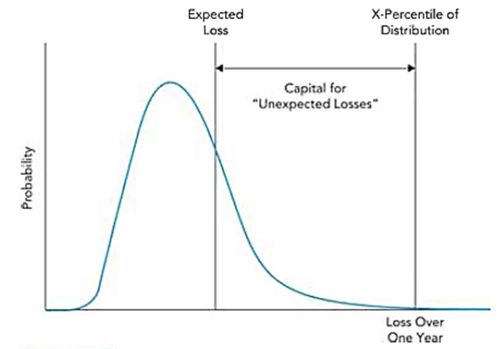
• The model used to estimate both economic capital and regulatory capital for credit risk is illustrated in this figure. The figure shows the probability distribution of default losses during a one-year period. The expected loss (i.e., the mean of the distribution) and a high percentile (X%) of the loss distribution are indicated.

• Expected loss the loss that a expects and it sets interest rates on its loans considering that loss. EL (in percentage terms is calculated as

     EL = PD × LGD or EL = PD × (1-RR)

If the expected default rate on the bank’s loan portfolio is 1.5% and the recovery rate in the event of a default is 40%, the expected loss is 0.9%.

• As a simple case, assume that the bank in the previous example (PD=1.5% and RR=40%) charges just enough on its loans to cover expected losses on the loans, the expenses involved in managing and administering the loans, and the cost of funding the loans. Suppose the bank needs a margin of 1.6% on its lending to cover its expenses. The total margin to cover its expected losses and expenses is therefore

1.6% + 0.9% = 2.5%

If the bank’s average funding cost is 1%, the average interest rate it charges on its loans needs to be

2.5% + 1% = 3.5%

• A challenge in managing credit risk is that actual losses do not equal expected losses every year The 0.9% default loss on the loan portfolio in our example is simply an average. In some years, losses will be less than this; in other years, they will be greater. The bank’s capital is a cushion that covers the unexpected loss. Using the VaR terminology, the required capital is the expected loss subtracted from the VaR with a one-year time horizon and an X% confidence level.

• The Basel Committee sets X=99.9% for regulatory capital in the internal ratings-based approach. This is because it wants the capital for credit risk to cover losses 99.9% of the time. To put this another way, bank supervisors require capital to be sufficient for losses that (in theory) occur only once every thousand years.

• When banks determine economic capital, they tend to be even more conservative. Consider a bank rated as AA. One of its key objectives will almost certainly be to maintain its AA credit rating. On an average, an AA-rated corporation has a default probability of about 0.02% in one year. A bank can maintain an AA rating if it is able to convince rating agencies there is 99.98% probability that it will not default. One way of doing this is by setting X as high as 99.98%. The capital is then theoretically sufficient to absorb losses in 4,999 out of 5,000 years.

Mean and Standard Deviation of Credit Losses

• Suppose a bank has n loans, and define the following quantities:

1. L_i : The amount borrowed in the i^th loan (assumed constant throughout the year)

2. p_i : The probability of default for the i^th loan

3. R_i : The recovery rate in the event of default by the i^th loan (assumed known with certainty)

4. ρ_ij : The correlation between losses on the i^th and j^th loan

5. σ_i The standard deviation of loss from the i^th loan

6. σ_P: The standard deviation of loss from the portfolio

7. α: The standard deviation of portfolio loss as a fraction of the size of the portfolio

• This table and figure displays the relationship between α and ρ. As expected, α increases as ρ increases.  The rate of increase is greatest for small values of ρ.

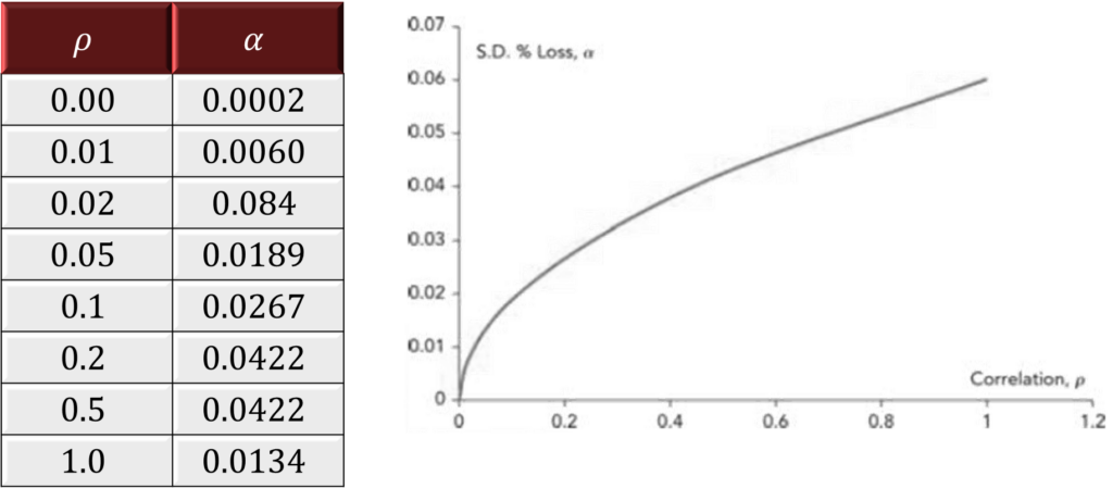
• To calculate bank capital using the model correlations have to be estimated first. Then the unexpected loss is estimated. Correlations can be estimated from a bank’s historical data. Also, rating agencies estimate the correlations between the default rates of two companies as a function of their rating.

• The calculation of unexpected loss requires an estimate of a high percentile of the loss distribution. There is no easy way to obtain this, however, and so the Monte Carlo simulation is often employed. On each simulation, random sampling determines whether each debtor defaults during a one-year period, and the results for many trials determine a probability distribution for default losses during the year.

The Gaussian Copula Model

• The Gaussian copula model is used in both bank and regulator models.

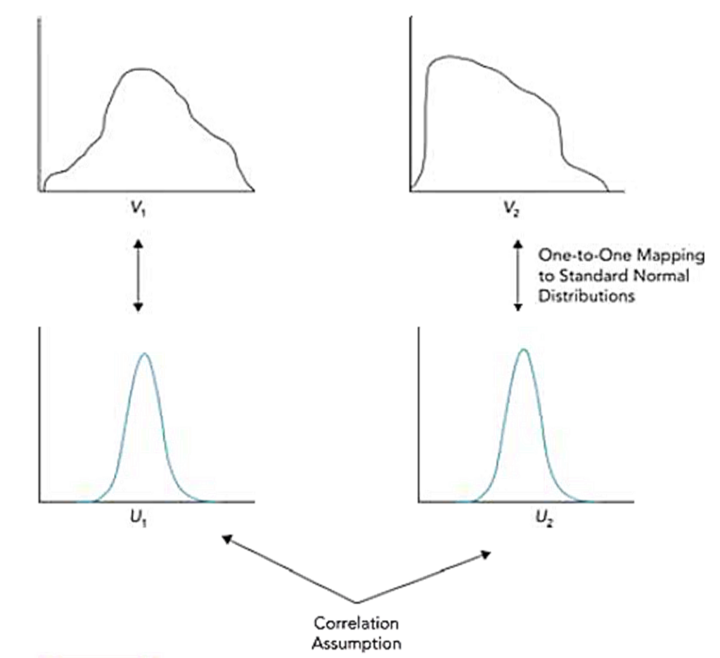
• If probability distributions for variables V₁ and V₂ are known to be normal, then the joint distribution can be assumed as bivariate normal. If their distributions are not normal, each distribution can be transformed to a standard normal distribution by transforming  their percentiles to the corresponding percentiles of a standard normal distribution.

• Lets assume V₁  is transformed to U₁ and V₂ is transformed to U₂, where U₁ and U₂ are (by construction) normal distributions with mean zero and standard deviation one. The one-percentile point on the distribution for V₁ is transformed to the one-percentile point of the distribution for U₁ (i.e., −2.326), the five-percentile point on the distribution  for V₁ is transformed to the five-percentile point on the distribution for U₁ (i.e., −1.645), and so on. Similarly, the one-percentile point on the distribution for V₂ is transformed to U₂ = −2.326, the five-percentile point on the distribution for V₂ is transformed to U₂ = −1.645, and so on.

• Then the distributions of U₁ and U₂  are assumed to be bivariate normal with a particular correlation. This defines the joint distribution of U₁ and U₂.

• The issue of defining the correlation between the U_i  distributions can be challenging. When there are many different distributions, this involves specifying a large number of different correlation parameters. Analysts often handle this problem by using a one-factor model. A one-factor model assumes that:

where

F is a factor common to all the U_i.

Z_i is the component of U_i that is unrelated to the common factor F.

The Z_i corresponding to the different U_i are uncorrelated with each other.

The variables F and Z_i have standard normal distributions (i.e., normal distributions with mean zero and standard deviation 1).

a_i are parameters with values between –1 and +1.

The variable U_i is the sum of two independent normal distributions and is therefore normal. It has a mean of zero because it is the sum of two components, each of which has a mean of zero.

• An example of a one-factor model is the capital asset pricing model (CAPM). In this model, the correlation between the returns from two stocks is assumed to arise entirely from their dependence on a common factor. In the case of CAPM, the common factor is the return from the market index. CAPM is an approximation. For example, there is presumably some correlation between the return from General Motors and the return from Ford that is unrelated to their correlation with the market index. However, CAPM makes the specification of correlations between the returns from different stocks easy to handle.

• The one-factor model can be applied to default probabilities. The factor can be thought of as a variable related to the economy that affects default rates.

The Vasicek Model

• The Vasicek model is used by regulators to determine capital for loan portfolios. It uses the Gaussian copula model to define the correlation between defaults. The Vasicek model has the advantage that the unexpected loss can be determined analytically. The probability of default (PD) is assumed to be same for all companies in a large portfolio.

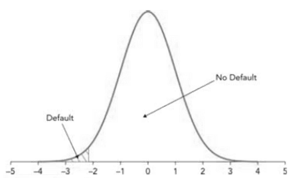
• The binary probability of the default distribution for company i for one year is mapped to a standard normal distribution U_i as described in the previous section. Values in the extreme left tail of this standard normal distribution correspond to a default, whereas the rest of the distribution corresponds to no default.. Company i therefore defaults if:

where 

N^-1 is the inverse cumulative normal distribution.

For example, if PD=1%, company i defaults if:

Values for U_i between minus infinity and –2.326 correspond to default, while values between –2.326 and infinity correspond to no default.

• The one-factor model defines the correlation between defaults. To make the model manageable for a loan portfolio, the ai are assumed to be the same for all i. Setting a_i=a, the model becomes

and so  the correlation between each pair of U-distributions is a².

• The factor F can be thought of as an index of the recent health of the economy.

1. If F is high, the economy is doing well and all the U_i will tend to be high (making defaults unlikely).

2. If F is low, however, all the U_i will tend to be low so that defaults are relatively likely.

• For each value of F, the distribution of each U_i has a mean of aF and a standard deviation of √(1-a² ). For a large portfolio, the default rate is the probability U_i is less than N^-1 (PD). From the properties of normal distributions,

	PD=0.1%	PD=0.5%	PD=1%	PD=1.5%	PD=2%
ρ=0.0	0.1	0.5%	1.0%	1.5%	2.0%
ρ=0.2	2.8	9.1%	14.6%	18.9%	22.6%
ρ=0.4	7.1	21.1%	31.6%	39.0%	44.9%
ρ=0.6	13.5%	38.7%	54.2%	63.8%	70.5%
ρ=0.8	23.3%	66.3%	83.6%	90.8%	94.4%

• The 99.9 percentile of the default rate increases with both the PD and the ρ, as seen above.

• The Vasicek model can be used to find the unexpected loss for a loan portfolio. Consider a portfolio of loans with the same PD, the same ρ, the same loss given default (LGD), and the same principal. The Basel II capital requirement for banks that use the IRB approach is:

where 

WCDR (worst case default rate) is the 99.9 percentile of the default rate distribution given by

LGD is the loss given default (equals one minus the recovery rate), and

EAD is the total exposure at default (i.e., the sum of the principals of all the loans).

The above equation gives the unexpected loss with a 99.9% confidence level. This is because WCDR × LGD is the 99.9 percentile point of the loss rate distribution, and WCDR×LGD×EAD is the loss at this 99.9 percentile point. Similarly, PD×LGD×EAD is the expected loss.

Creditmetrics

• Credit Metrics is the model banks often use to determine economic capital. Under this model, each borrower is assigned an external or internal credit rating. A one-year transition table is used to define changes in ratings. The bank’s portfolio of loans is valued at the beginning of a one-year period. A Monte Carlo simulation is then carried out to model how ratings change during the year. In each simulation trial, the ratings of all borrowers at the end of the year are determined, and the portfolio is revalued. The credit loss is calculated as the value of the portfolio at the beginning of the year minus the value of the portfolio at the end of the year. The results of many simulation trials are used to produce a complete credit loss distribution.

Transition	Probability
′′B^′′ to ′′A′′	0.05
stays “B”	0.80
′′B^′′ to ′′A′′	0.13
Defaults	0.02

• Credit Metrics model can be illustrated with a simple example. Suppose a bank uses four ratings: A, B, C, and default. As indicated in Table 6.4, a B-rated borrower has a 5% chance of being upgraded to A during the year, an 80% chance of staying at a B, a 13% chance of being downgraded to C, and a 2% chance of defaulting.

• On each simulation trial, a number is sampled from a standard normal distribution to determine what happens to a given B-rated borrower. Since

the rules that are implemented are shown in the following table. These rules ensure the transition probabilities in the previous table apply.

Sample Range	Rating Transition
Less than -1.645	′′B^′′ to ′′A′′
Between -1.645 and 1.036	stays “B”
Between 1.036 and 2.054	′′B^′′ to ′′A′′
Greater than 2.054	Defaults

Risk Allocation

• Euler’s result can be used to divide many of the risk measures used by risk managers into their component parts. It is concerned with what are termed homogeneous functions. These are functions, F, of a set of variables x₁, x₂, …,x_n having the property:

for a constant λ.

Define

where

∆x_i is a small change in variable i, and

∆F_i is the resultant small change in F.

Here, Q_i is the ratio of ∆F_i  to a proportional change, ∆x_i / x_i , in x_i. Euler showed that in the limit, as the size of the ∆x_i tends to zero:

• Many risk measures are homogeneous functions. In fact, homogeneity is one of the properties of a coherent risk measure. If a portfolio is changed so that each position is multiplied by some constant λ, a risk measure is usually multiplied by λ. Euler’s theorem therefore gives a way of allocating a risk measure F that is a function of many different trades into its component parts.

• In the context of credit risk, Euler’s theorem can be used to determine the contribution of each loan in a portfolio to the overall risk measure. To illustrate this, let us take a very simple example.

	Loan 1	Loan 1	Loan 1
Loan 1	1	0	0
Loan 1	0	1	0.7
Loan 1	0	0.7	1

Derivatives

• Derivatives also give rise to credit risk. The equation UL=(WCDR-PD)×LGD×EAD for unexpected losses can be used to calculate credit risk capital for derivatives as well as loans. But a problem in using them for derivatives is that it is difficult to calculate EAD for a derivatives transaction. In the case of a loan, EAD is usually the amount that has been advanced (or is expected to be advanced) to the borrower. In the case of a derivative, the exposure varies from day to day as the value of the derivative changes. The Basel Committee’s standard rules for determining EAD have solved this problem by setting the exposure at default for derivatives equal to the current exposure plus an add-on amount. The current exposure is the maximum amount that could be lost if the counterparty defaulted today. The add-on amount is an allowance for the possibility of the exposure getting worse by the time a default occurs.

• Another challenge is that derivatives are subject to netting agreements. This means all outstanding derivatives with a counterparty may be considered a single derivative in the event that the counterparty defaults. This means that the equation cannot be used on a transaction-by-transaction basis. Instead, it must be implemented on a counterparty by- counterparty basis.

Challenges

• The assessment of credit risk requires many estimates (e.g., PD). Just as the distinction between through-the-cycle and point-in-time for credit ratings can be made, a distinction between a through-the-cycle PD and a point-in-time PD can also be made.

1. A through-the-cycle PD is an average PD over an economic cycle, whereas a point-in-time PD reflects current economic conditions.

• Regulators require banks to estimate a through-the-cycle PD for regulatory capital purposes. However, point-in-time estimates might be more appropriate for internal purposes.  A further complication is that accounting standards (such as IFRS 9) require loans to be valued for accounting purposes. Expected losses (either over one year or during the loan’s life, depending on the situation) must be calculated and subtracted from the principal amount of the loan. For this purpose, a point-in-time estimate is required.

1. Banks are therefore faced with the problem of making both through-the-cycle estimates (to satisfy regulators) and point-in-time estimates (to satisfy their auditors).

• Another required estimate is the recovery rate (or loss given default). The recovery rate is negatively correlated with the default rate. Thus, an economic downturn is doubly bad for credit risk because the default rate increases, and the recovery rate decreases.

• A further estimate is exposure at default. This is the amount the borrower owes at the time of default. For a portfolio of derivative transactions, a relatively complex calculation is required to determine the expected exposure during a year. A consideration might be what is termed wrong-way risk. This is the risk associated with the fact that a counterparty to a company may be more likely to default when the value of outstanding derivatives is negative to the company (and therefore positive to the counterparty).

• Correlations are difficult to estimate. The Gaussian copula model is easy to use, but there is no guarantee it reflects just how bad loan losses would be in a one-in-a-thousand years scenario (or in the case of economic capital, an even more extreme scenario).

• Apart from credit, the bank also must worry about market risk, operational risk, liquidity risk, strategic risk, and so on. These risks tend to be handled by different groups within a bank, but they are not independent of each other. They interact and influence the bank’s total required capital (both regulatory and economic).