Introduction to Operational Risk

• There are many ways operational risk can be defined. It is sometimes defined very broadly as any risk that is not a market risk or credit risk. A much narrower definition is that – it consists of risks arising from operational mistakes, including the risk that a bank transaction is processed incorrectly, but excluding the risk of fraud, cyberattacks, or damage to physical assets.

• Operational risk has been defined by the Basel Committee as –

“The risk of loss resulting from inadequate or failed internal processes, people, and systems or from external events.”

• The International Association of Insurance Supervisors defines operational risk similarly as –
“The risk of adverse change in the value of capital resources resulting from operational events such as inadequacy or failure of internal systems, personnel, procedures or controls, as well as external events.”

• These definitions include the risks arising from computer hacking, fines from regulatory agencies, litigation, rogue traders, terrorism, systems failures, and so on. However, they do not  include strategic risks or reputational risks.

Categories of Operational Risk

• According to Basel committee, operational risk can be categorized into following seven categories –

1. Internal fraud – Acts intended to defraud, misappropriate property, or circumvent regulations, the law, or company policy involving at least one internal party. Examples include intentional misreporting of positions, employee theft, and insider trading.

2. External fraud – Acts, by a third party, intended to defraud, misappropriate property, or circumvent the law. For example, robbery, forgery, check kiting, and computer hacking.

3. Employment practices and work-place safety – Acts inconsistent with employment, health or safety laws or agreements, or which result in payment of personal injury claims, or claims relating to diversity or discrimination issues. For example, workers compensation claims, violation of employee health and safety rules, discrimination claims.

4. Clients, products, and business practices – Unintentional or negligent failure to meet a professional obligation to clients and the use of inappropriate products or business practices. For example, fiduciary breaches, misuse of confidential customer information, money laundering, and the sale of unauthorized products.

5. Damage to physical assets – Loss or damage to physical assets from natural disasters or other events. For example, terrorism, vandalism, earthquakes, fires, and floods.

6. Business disruption and system failures – For example, hardware and software failures, utility outages, and telecommunication problems.

7. Execution, delivery, and process management – Failed transaction processing or process management, and disputes with trade counterparties and vendors. For example, data entry errors, collateral management failures, incomplete legal documentation.

Large Risks – Cyber Risks

• Financial Institutions and their clients have benefited from the development of credit and debit cards, online banking, mobile wallets, electronic funds transfer, and so on. However, these innovations have also created opportunities for cyber crime.

• Cyber crime includes the theft of money, intellectual property, personal and financial data, etc. Such crimes can also include destruction of data, embezzlement, fraud, and so on. Large corporations are under continuous attack by cyber criminals. Most are unsuccessful, but the number of successful attacks are rising each year. In addition, there may be many successful attacks that go unreported.

• Cyber threats can come in the form of individual hackers, nation states, organized crime, and even insiders. So, defenses such as user account controls, cryptography, intruder detection software, and firewalls must be developed to combat such threats.

• It is important that companies come to terms with the fact that even with the deployment of extremely sophisticated defenses, there will always be a real threat of becoming victim to a cyber attack. Thus, with the prevention plans in place, emphasis must also fall on damage control in the scenario where the cyber defenses of the company are breached. The companies must have plans that can be implemented on short notice, to deal with attacks of different severities. In some instances, an extreme response to an attack, such as delaying the acceptance of new transactions for a few days, might become necessary.

Large Risks – Compliance Risks

• Compliance risk is the risk that an organization would incur fines or other penalties due to its, knowing or unknowing, failure to act in accordance with industry laws and regulations, internal policies, or prescribed best practices. Activities such as money laundering, terror financing, and assisting clients with tax evasion can all lead to big penalties. For instance, Volkswagen was fined due to its failure to comply with US emission standards, while HSBC and BNP Paribas were fined by US law agencies due to their non-compliance with money laundering laws.

• Though regulatory infractions can result from a small part of a large company’s global activities, they can be very expensive (both in terms of fines and loss of reputation). It is important for financial institutions to have systems in place to ensure that they are following all applicable laws and regulations. In this regard, technology can be of great help. For example, some banks have developed systems designed to detect suspicious requests to open accounts or transfer funds in real time.

Large Risks – Rogue Trader

• The risk of rogue trading has been sensationalized in the various finance movies over the last decade or so. This is essentially the risk a company faces when an employee takes unauthorized actions or trades resulting in large losses. Some notable examples are – Barings Bank trader Nick Leeson, whose unauthorized trading activities led to a loss of USD 1 billion that resulted in the collapse of the bank in 1995. In a similar breach of norms by a trader named Jerome Kerviel, Société Générale incurred a loss of EUR 4.9 billion due to Kerviel’s trading activities.

• One thing a bank can do to protect itself from rouge trading is to ensure that the front office (which is responsible for trading) is totally independent of the back office (which is responsible for record keeping and verifying transactions).

• A more complicated issue is the way in which unauthorized trading is treated when it is uncovered. If a trader conducts unauthorized trading and takes a loss, there are likely to be unpleasant consequences for the trader. But the complications arise when the trader makes a large profit by taking a huge unauthorized risk. In such a scenario, the company might be tempted to ignore the violations. This is a short-sighted approach however, as it leads to a culture where risk limits are not taken seriously. This in turn paves the way for disaster.

Basel II Regulations

• The Basel Committee on Banking Supervision develops global regulations, which are then implemented by bank supervisors in each member country. In 1999, Basel II was drafted, which was a revision of the methods for calculating credit risk capital. It also included the approaches to determine the operational risk capital.

• Many risk managers deemed capital requirements for operational risk to be unworkable due to the difficulty in quantifying operational risk. Even if operational risks could not be quantified precisely, Basel Committee considered it important for banks to devote more resources toward managing them.

• There has been a parallel development in the regulation of insurance companies. Insurance regulators use a definition of operational risk similar to that used by Basel II.

• The final Basel II rules for banks had three approaches:

1. The basic indicator approach,

2. The standardized approach, and

3. The advanced measurement approach (AMA).

Basel II Regulations – Basic Indicator Approach

• In the basic indicator approach, operational risk capital is set equal to 15% of the three-year average annual gross income. Gross income is defined as:

Gross Income = Interest earned – interest paid + non-interest income

Basel II Regulations – Standardized Approach

• The standardized approach is like the basic indicator approach, except that separate calculations are carried out by each business line and the percentage applied to gross income varies across business lines. The percentages for eight business lines are given in the table below.

Business Line	Capital (% of Gross Income)
Corporate finance	18%
Trading and sales	18%
Retail banking	12%
Commercial banking	15%
Payment and settlement	18%
Agency services	15%
Asset management	12%
Retail brokerage	12%

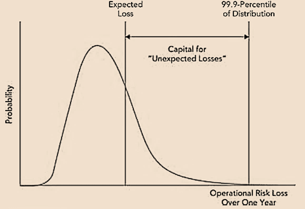
Basel II Regulations – Advanced Measurement Approach

• The AMA in Basel II is much more complicated than the other two approaches. Banks are required to treat operational risk like credit risk and set capital equal to the 99.9 percentile of the loss distribution minus the expected operational loss. The model can be illustrated using the figure.

• Under the AMA approach, banks are required to consider every combination of the eight business lines mentioned in the table in standardized approach and the seven categories of operational risk. For each of the 56 (=7×8) combinations, they had to estimate the 99.9 percentile of the loss. These estimates are then aggregated to determine the total capital requirement.

• The Basel Committee has now abandoned AMA and is replacing all three of the approaches in Basel II with a new standardized approach. However, many banks still use it as part of their economic capital determinations.

• The AMA operational risk methodology has proved useful in prompting financial institutions to think more about the operational risks they face. However, bank regulators have found the approach unsatisfactory due to the high degree of variation in the calculations carried out by different banks. Two banks presented with the same data were liable to come up with quite different capital requirements under AMA.

Revision to Basel II – Standardized Measurement Approach

• On March 2016, the Basel Committee announced the replacement of all previous approaches for determining operational risk capital with the standardized measurement approach (SMA).The SMA first defines a quantity known as the Business Indicator (BI). BI is like gross income, but it is designed to be a more relevant measure of bank size. For example, items such as trading losses and operating expenses are treated differently so that they increase BI.

• The Bl Component for a bank is calculated from the BI using a piecewise linear relationship. A loss component is then calculated as:

7X + 7Y + 5Z

where,

X is average of all losses from operational risk over past 10 years,

Y is average of losses greater than EUR 10 million from operational risk over past 10 years,

Z is average of losses greater than EUR 100 million from operational risk over past 10 years.

• The calculations are designed so that the loss component and the BI Component are equal for an average bank. The Basel Committee provides a formula for calculating required capital from the loss and the BI component.

Determining the Loss Distribution

• Economic capital calculations require a distribution, like that in figure discussed is AMA approach, for several categories of operational risk losses and the combined results.

• The key determinants of an operational risk loss distribution are –

1. Average Loss Frequency

2. Loss Severity

Determining the Loss Distribution – Loss Frequency

• The Average Loss Frequency is the average number of times in a year that large losses occur. A Poisson distribution is often assumed for loss frequency. If the expected number of losses in a year is λ, the probability of n losses during the year given by the Poisson distribution is –

• The parameter λ is equal to the average number of losses in each time period. If, 12 losses occur over 3 years, then average number of losses per year (λ) will be equal to –

λ = 12/3 = 4

• And the probability that there will be exactly 3 and 10 losses in a year can be found as –

And,

Determining the Loss Distribution – Loss Severity

• Loss Severity is the probability distribution of the size of each loss. The mean and standard deviation of the loss severity is often fitted to a lognormal distribution.

• Suppose the mean and standard deviation of the loss size are estimated to be μ and σ, respectively. Also, suppose the mean of the logarithm of the loss size is μ_1 and variance of the logarithm of the loss size is σ_1^2. Then, under the lognormal assumption,

 where, w = σ/μ²

• Suppose the mean and standard deviation of the loss size are estimated (in USD million) as 80 and 40, then,  w=(40/80)^2=0.25

The logarithm of the loss size therefore has a mean and variance of –

Determining the Loss Distribution – Monte Carlo Simulation

• Once λ, μ and σ have been estimated, a Monte Carlo simulation can be used to determine the probability distribution of the loss. The general approach is illustrated in the figure below.

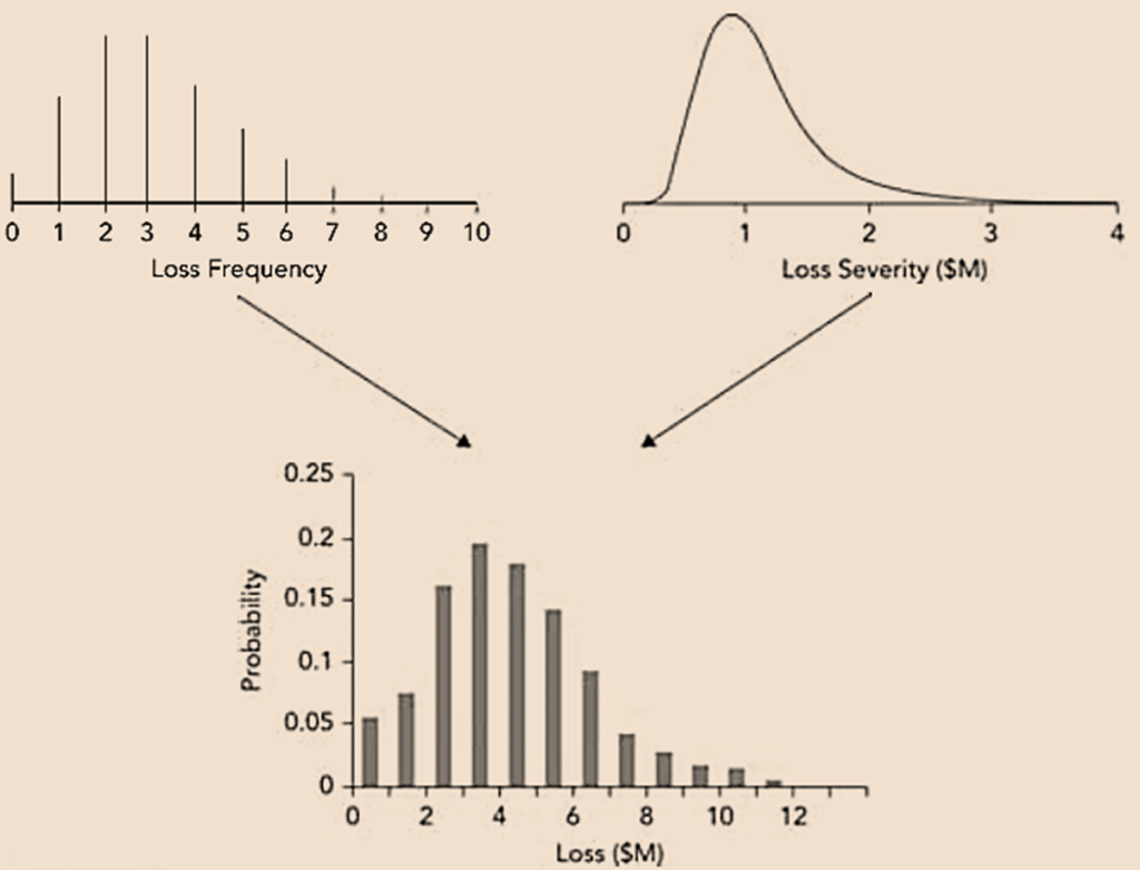
• The steps in the procedure are as follows –

1. Step 1 – Sample from the Poisson distribution to determine the number of loss events(n)in a year. For example, the percentile of the Poisson distribution can be sampled as a random number between 0 and 1.

2. Step 2 – Sample n times from the lognormal distribution of the loss size for each of the n loss events.

3. Step 3 – Sum the n loss sizes to determine the total loss.

4. Step 4 – Repeat steps 1 to 3 many times.

• Suppose that the average loss frequency is 4 and the random number sampled is 0.31. This corresponds to three loss events. This can be shown as follows –

And,

Using the formula

Therefore,

• The sampled number 0.31 lies between these two cumulative probabilities.

• Suppose the loss size has mean 80 and standard deviation 40. The mean and variance of the logarithm of loss size has already been found previously as 7.959 and 0.223.

• For step 2, we sample three times from a normal distribution with mean 7.959 and variance 0.223. If the numbers sampled are 4.1, 5.1, and 4.4, the three losses are

e^4.1  = 60.34

e^5.1=164.02

e^4.4  = 81.45

• Step 3 gives the total loss on that simulation trial of 305.81 ( = 60.34 + 164.02 + 81.45).

• By carrying out many Monte Carlo  simulation trials such as this, we obtain a probability distribution for the total loss from which the required percentile can be calculated.

Determining the Loss Distribution – Estimation Procedures

• The historical data on operational risk losses is scarce. So, estimating the loss frequency and loss severity for a category of losses involves a combination of data and subjective judgement. Loss frequency should be estimated either from a bank’s own data or subjectively by operational risk professionals after careful consideration of the controls in place.

• When loss severity cannot be estimated from a financial institution’s own data, the losses experienced by other financial institutions can sometimes be used as a guide. Mechanisms for sharing loss data between banks have been developed. Additionally, data vendor services (such as Factiva and Lexis-Nexis) can be useful in providing data on publicly reported losses experienced by other banks.

Determining the Loss Distribution – Potential Biases

• Data from data vendors can potentially be biased because only large losses are usually reported. If the data from a vendor is used in a direct way to determine the loss severity distribution, the distribution is likely to be biased toward large losses.

• This bias can be avoided if the data is used to determine only relative loss severity. If data from a vendor indicates Loss Type A (on which a bank has no data) is on average twice as severe as Loss Type B (on which the bank does have data), the bank might assume that the mean loss for Loss Type A is twice that calculated using its own data for Loss Type B.

• Another potential bias concerns the size of loss. If Bank B has revenue of USD 20 billion and experiences a loss of USD 300 million. Bank A, with revenues of USD 10 billion, is using this loss event to estimate the severity of a similar loss it might incur. Bank A’s loss would most likely not be as large as USD 300 million as it is a smaller bank than Bank B. But it would be too optimistic to estimate its loss to be half of that of Bank B. The relationship can be approximated as –

• It is estimated that β=0.23 gives a good fit. The loss for Bank A in the previous example would therefore be –

or USD 256 million.

• It is also important to adjust loss severity estimates for inflation. A loss of a certain size observed ten years ago can be expected to be larger if the same set of circumstances repeat themselves.

Determining the Loss Distribution – Scenario Analysis

• Financial institutions also use scenario analysis to estimate loss frequencies and loss severities. It is particularly useful for loss events with a low frequency but high severity. These are the important loss events because they tend to determine the extreme tails of the loss distribution.

• This approach tries to list these events and generate a scenario for each one. The scenarios might come from a financial institution’s own experience, known experience of other banks, hypothetical scenarios generated by risk management professionals, and consultants.

• For each scenario, loss frequency and loss severity estimates are made. Monte Carlo simulations are used to determine a probability distribution for total loss across different categories of losses. The loss frequency estimate should reflect the controls in place at the financial institution and the type of business.

• Probability estimation of rare events is difficult. One approach is to specify several categories and ask operational risk experts to assign each loss to a category. The categories could be, Scenario that happens once every 1,000 years on average (λ=0.001), Scenario that happens once every 100 years on average (λ=0.01), and so on.

• Operational risk experts must also estimate loss severity. Rather than estimate the mean and standard deviation, it might be more appropriate to ask for estimates of the 1 percentile to 99 percentile range of the loss distribution. These estimates can be made to fit to a lognormal distribution.

• Suppose that 20 and 200 are the 1 percentile and 99 percentile of the loss (respectively). Then ln⁡(20)=2.996 and ln⁡(200)=5.298 are the 1 and 99 percentiles for the logarithm of the loss distribution (respectively). From this, it follows that the logarithm of the loss distribution has a mean (μ) and standard deviation (σ) of –

• Scenario analysis considers losses that have never been experienced by a financial institution yet but could happen in the future. Managerial judgement is used to assess loss frequency and loss severity which leads to a discussion about how such loss events can occur. This can help firms form strategies for responding to a loss event and/or reduce the probability of it happening.

Reducing Operational Risk – Causes of Losses

• Sometimes operational risk losses can be related to other factors that can be managed. For example, in some situations it might be possible to show that losses can be reduced by increasing employee training or the educational qualifications necessary for a certain position. In other situations, it might be possible to show losses arising from an outdated computer system.

• It is not always the case that operational risk losses should be minimized. A cost-benefit analysis should be undertaken because the costs of reducing operational risk can sometimes outweigh the benefits.

Reducing Operational Risk – Risk Control and Self Assessment

• Risk Control and Self Assessment (RCSA) is one way in which financial institutions try to understand operational risks while creating an awareness of operational risk among employees. Line managers and their staff are asked to identify risk exposures. The risks considered should include not just losses that have occurred in the past, but the potential future losses also. Some RCSA approaches include –

1. interviewing line managers and their staff

2. asking line managers to complete risk questionnaires

3. reviewing risk incident history with line managers

4. reviewing third-party reports such as those of auditors, regulators, and consultants

5. reviewing reports of the experiences of similar managers in other companies

6. using of suggestion boxes and intranet reporting portals

7. implementation of a ‘whistle blowing’ process to encourage the reporting of risk issues

8. carrying out brainstorming in a workshop environment

• The assessment process should be repeated periodically. The frequency of loss events and their severity should be quantified. Some loss events are inevitable in business. For others, the RCSA leads to improvements by reducing the frequency of losses, severity of losses, or both.

Reducing Operational Risk – Key Risk Indicators

• A developed understanding of the risks faced by line managers can lead to the development of key risk indicators (KRIs). These are data points that may indicate a heightened chance of operational risk losses in certain areas. In some cases, remedial action can be taken before it is too late. Simple examples of KRIs are metrics related to-

1. Staff turnover

2. Failed transactions

3. Positions filled by temps

4. Unfilled positions

• To use these indicators effectively, it is important to track how they change through time so that unusual behavior can be identified. Some KRIs are subtler than others. For example, the unwillingness of an employee to take vacations might be an indication that he or she could be engaged in unauthorized trading or embezzling funds.

• Using tools such as surveillance software to search for unusual email or phone activity indicative of an employee engaging in unlawful or unethical activity, can be useful in this regard.

Reducing Operational Risk – Education

• Employee education can be important in reducing operational risk. Compliance is an area that can lead to huge operational risk losses. Educating employees about unacceptable business practices and creating a risk culture where such practices are perceived to be unacceptable is important.

• Legal disputes are unfortunately an inevitable part of doing business. In a legal dispute where an organization is being sued, the organization usually must provide all relevant internal communications. Some can be very embarrassing. So, the in-house legal department within a financial institution needs to remind employees to be careful about what they write in e-mails and (when they are recorded) what they say in phone calls.

• Before communicating via the use of emails or recorded phone calls, an employee should always consider whether he or she would be comfortable if the communication became public knowledge.

Allocation of Economic Capital

• Economic capital is allocated to business units so that a return on capital can be calculated. The procedure, similar to the allocation of credit risk capital, can (in principle) be used for allocating operational risk capital.

• The allocation of operational risk capital provides an incentive for a business unit manager to reduce operational risk. If the business unit manager can show that he or she has successfully reduced either loss frequency or loss severity, less capital will be allocated to the business unit. The unit’s return on capital will then improve and the manager can hope for a bigger bonus. The allocation process should sensitize the manager to the importance of operational risk.

• It is not always optimal to reduce operational risk. Some level of operational risk is inevitable in any business unit, and any decision to reduce operational risk by increasing operating costs should be justified with a cost-benefit analysis.

Power Law

• Economic capital is often calculated with very high confidence levels. For some probability distributions occurring in nature, it has been observed that a result known as the power law holds. If v is the value of a random variable and x is a high value of v, then the power law holds it is approximately true that –

where,

Pr⁡ denotes probability, and K and α are parameters.

• The power law describes how fat the right tail of the probability distribution of v is. The parameters K and α depend on the variable being considered. K is a scale parameter, while α reflects the fatness of the distribution’s right tail. As the parameter α decreases, this tail becomes fatter.

• The power law only describes the right tail of the distribution. That is why Equation given above is approximately true only for high values of x that are well into the right tail of the distribution of v.

• In general, it can be said that the power law holds for probability distributions of random variables which are the result of aggregating many independent random effects in some manner.

• Power law can hold for operational risk losses. This can be useful in some circumstances. For example, suppose K and α are estimated as 10,000 and 3 (respectively). In order to estimate the 99.5% percentile of the loss distribution (in USD millions), equation of power law can used to solve for x –

Insurance

• Many operational risks can be insured against. However, operational risk managers need to carefully evaluate whether the cost of insurance can be justified. The SMA for assessing operational risk is based on the frequency and magnitude of the losses incurred over the previous ten years. Thus, insuring against a loss can not only reduce the severity of losses, but also reduce capital requirements.

• To understand how insurance companies view operational risk, two key risks that they face must be reviewed. These are –

1. Moral Hazard

2. Adverse Selection

Insurance – Moral Hazard

• Moral hazard is the risk that the existence of an insurance contract will cause the insured entity to behave in a way that makes a loss more likely.

• One example of moral hazard concerns rogue trader losses. If an insurance company insures a bank against such losses, it might be concerned traders would take large unauthorized risks. If a gain resulted, the bank would be pleased. If a loss resulted, a claim would be made against the insurance company.

• In practice, insurance companies manage the moral hazard by carefully specifying trading limits and often requiring that the policies are not revealed to traders. Any losses incurred are investigated carefully, and if financial institutions fail to follow their insurance requirements, they might forfeit their payout.

• Insurance companies manage moral hazard by using deductibles so that a financial institution is responsible for the first part of any loss. There may also be a co-insurance provision where the insurance company pays only a percentage of a loss. There is always a limit on the total amount that can be paid. Insurance premiums may also increase after a loss has been incurred.

Insurance – Adverse Selection

• Adverse selection is the problem an insurance company faces in distinguishing low-risk situations from high-risk situations. If it charges the same premium for a certain type of risk to all financial institutions, it will inevitably attract clients with the highest risk.

• For example, if all banks were offered the same insurance premiums to insure against rouge trader losses, banks with poor internal controls would tend to buy more insurance, while those with good internal controls would consider the cost of the insurance too high (and therefore buy less insurance).

• Insurance companies deal with adverse selection by researching about potential customers before providing a quote. In the case of rogue trader insurance, a financial institution must convince an insurance company that it has good risk controls in place before it can qualify for insurance.