What is key rate exposure ?

Key rate exposure measures a portfolio's sensitivity to changes in interest rates at specific maturities.

How is principal components analysis used in finance ?

Principal components analysis helps understand term structure movements by identifying uncorrelated factors in historical rate data.

DV01, or dollar value of a basis point, measures the change in a portfolio's value for a one-basis-point shift in interest rates.

How are forward-bucket 01s calculated ?

Forward-bucket 01s are calculated by shifting forward rates within specific time buckets and measuring the portfolio's value change.

What is the difference between spot rate and par yield KR01s ?

Spot rate KR01s measure sensitivity to spot rate shifts, while par yield KR01s focus on changes in par yields.

What is the advantage of using the bucketing approach in hedging ?

The bucketing approach simplifies hedging by focusing on specific segments of the interest rate term structure.

How does multi-factor hedging improve risk management ?

Multi-factor hedging addresses various term structure movements, offering more comprehensive protection than single-factor hedging.

How can portfolio volatility be estimated using key rate analysis ?

Key rate analysis identifies sensitivity to interest rate shifts, helping estimate potential portfolio volatility.

What is the significance of duration measures in hedging ?

Duration measures the sensitivity of a portfolio’s value to interest rate changes, aiding in risk management.

How do forward rates affect bond pricing ?

Forward rates impact bond pricing by determining the present value of future cash flows, influencing the bond's sensitivity to rate changes.

Modeling Non-Parallel Term Structure Shifts And Hedging

Introduction

Describe the key rate exposure technique in multi-factor hedging applications; summarize its advantages and disadvantages.
Calculate the key rate exposures for a given security, and compute the appropriate hedging positions given a specific key rate exposure profile.
Relate key rates, partial ’01s and forward-bucket ’01s, and calculate the forward-bucket ’01 for a shift in rates in one or more buckets.
Apply key rate and multi-factor analysis to estimating portfolio volatility.

Principal Components Analysis

A statistical technique known as principal components analysis can be used to understand term structure movements in historical data. This technique looks at the daily movements in rates of various maturities and identifies certain factors. These factors are term structure movements with the property that:

The daily term structure movements observed are a linear combination of the factors (e.g., an observed movement might consist of five units of the first factor, two units of the second factor, and one unit of the third factor);
The factors are uncorrelated; and
The first two or three factors account for most of the observed daily movements.

A principal components analysis finds multiple factors and estimates their relative importance in describing movements in the term structure.
Example-

The Federal Reserve Board provides daily data on Treasury rates with maturities of 1, 2, 3, 5, 7, 10, 20, and 30 years. This data from the ten-year period between January 2008 and December 2017 can be used to carry out a principal components analysis on the daily changes in these eight rates. The number of factors equals the number of rates. Factor loadings are shown in this table. These are the amount by which each of the rates moves when there is one unit of the factor.

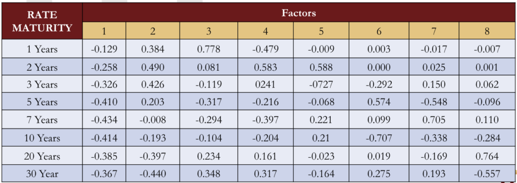
The factors are listed in order of importance (Factor 1 is the most important factor, Factor 2 is next most important, and so on). When there is +1 unit of Factor 1, the one year rate changes by -0.129 basis points, the two-year rate changes by -0.258 basis points, and so on. When there is +1 unit of Factor 2 the one-, two-, three-, and five year rates move up while the seven-, ten-, 20-, and 30-year rates move down. When there is +1 unit of Factor 3, the first two and last two rates move up while the intermediate four rates move down.
If all the signs of all the factor loadings for a particular factor are changed, it does not change the analysis. For example, in the previous table, all the factor loadings for Factor 1 are negative. This means that +1 unit of Factor 1 will cause all rates to decrease and -1 unit of Factor 1 will cause all rates to increase. Now suppose that all the signs are changed so that the factor loadings for the rates with maturities 1, 2, 3, 5, 7, 10, 20, and 30 years are 0.129, 0.258, 0.326, 0.410, 0.434, 0.414, 0.385, and 0.367 (respectively). It is then the case that +1 unit of the new Factor 1 has the same effect as −1 unit of the old Factor 1 (and vice versa). Because +1 unit and -1 unit of a factor are equally likely, the model is unchanged.

Because there are eight rates and eight factors, the change on any particular day can be calculated as a linear combination of the factors. The change in the j^th rate has the form:

$\sum_{i=1}^8 a_i f_{ij}$

where

$f_{ij}$ is the factor loading for the $i^\text{th}$ factor and the $j^\text{th}$ rate, and

$a_i \ (1 \leq i \leq 8)$ is the number of units of the $i^\text{th}$ factor in the daily change being considered.

The $a_i$ are known as factor scores. They are different for each of the daily changes in the historical sample. The importance of a factor is measured by the standard deviation of its factor scores. For the data being considered, the importance of the $i^\text{th}$ factor is the standard deviation of $a_i$ across all the approximately 2,500 daily changes in the term structure during the 2008–2017 period, shown in this table.

Factors	1	2	3	4	5	6	7	8
	14.15	4.91	2.44	1.59	1.09	0.85	0.78	0.68

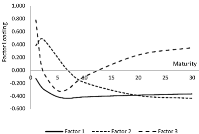
The factors can be seen to have the following properties :
- Factor 1 is a shift in the term structure where all rates move in the same direction by approximately (but not exactly) the same amount.
- Factor 2 is a shift where short-term rates move in one direction and long-term rates move in the other direction. It corresponds to steepening or flattening of the term structure.
- Factor 3 is a bowing of the term structure (i.e., where relatively short-term and relatively long-term rates move in one direction while intermediate rates move in the other direction).

Additionally, the variance of the factors scores add up to the total variance of all rate movements.

PARTIAL 01s

DV01 was defined as the impact of a one-basis point shift in all spot rates on the value of a portfolio. Suppose that three spot rates are considered : the two-year rate, the five-year rate, and the ten-year rate.

Let’s define –

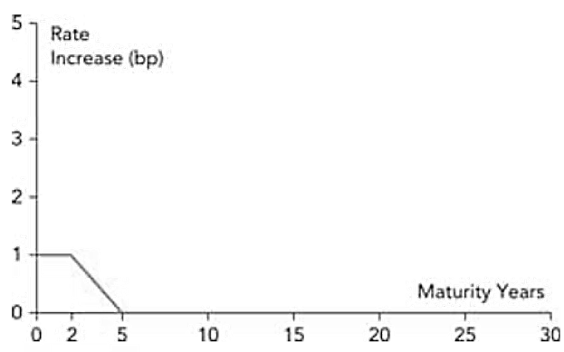
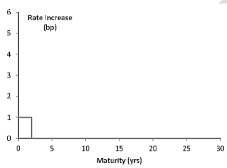
$KR01_1$ : The reduction in a portfolio’s value from a one-basis-point increase in the two-year spot rate, as shown in this figure

Let’s define –

$KR01_2$ : The reduction in a portfolio’s value from a one-basis-point increase in the five-year spot rate, as shown in this figure

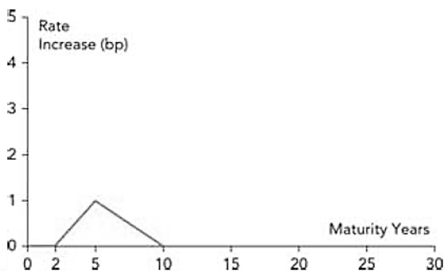
The shifts in the previous figures are sometimes referred to as key rate shifts. The combined effect of the three key rate shifts in those figures is a one-basis point shift in all rates. These figures therefore provide a way of splitting the DV01 measure into three other measures.
It follows that:

$\text{DV01}=\text{KR01}_1+\text{KR01}_2+\text{KR01}_3$

DV01 alone can be hedge against parallel shifts in the interest rate term structure. If an investor follows a similar procedure to hedge against $\text{KR01}_1, \text{KR01}_2, \text{KR01}_3$ the investor is hedged against a wider range of term structure movements. Specifically, the investor is hedged against small rate movements of the type shown in the previous figures as well as any combination of these three rate movements.

KR01s (either for a portfolio or for instruments used to hedge a portfolio) can usually be calculated in a fairly direct way from their sensitivities to spot rates. For example, suppose a portfolio consists of a USD 1 million investment in each of a one-year, three-year, five-year, nine-year, and 15-year zero coupon bond. Suppose, further that the term structure is flat at 3% (semi-annually compounded). The decrease in the portfolio’s value for a one-basis-point increase in the relevant spot rates is shown in this table.

Spot Rate Maturity (Years)	1	3	5	9	15
Portfolio Value Decrease	95.62	270.26	424.35	677.93	944.74

The exposures in the above table can be converted to exposures to the shifts in the previous figures. The following table shows the impact of the shifts in the previous figures on the five spot rates in the above table. For example, the shift in the two year rate involves a one-basis-point shift in the one-year rate and a 0.6667-basispoint shift in the three-year rate, with none of the other rates being affected.

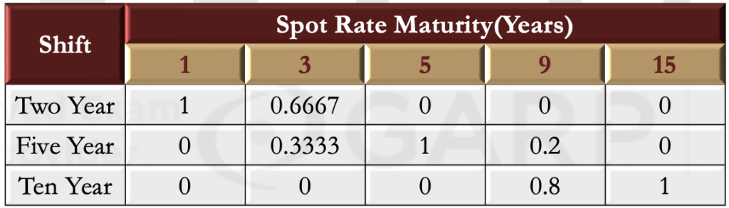
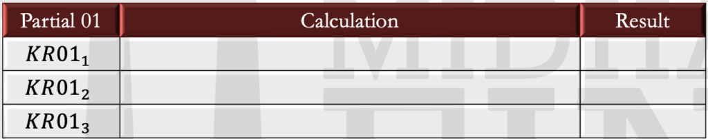
The KR01s for the portfolio with the exposures in can therefore be calculated as indicated in the following table

To obtain a hedge position, the data in the following table is used. This shows KR01s for a portfolio and three different hedging instruments.

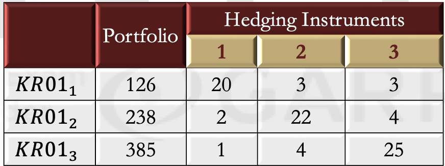
The positions in the three hedging instruments necessary to reduce the KR01s to zero can be calculated by solving three simultaneous equations. If $x_1, x_2, \text{and } \ x_3$ are the positions in the three hedging instruments –

Principal Components Analysis Revisited

Earlier, it was shown that the first three factors account for about 97.7% of the variance in Treasury rate movements over a ten-year period. Assuming the ten-year history is representative of future term structure movements, the portfolio is hedged against 97.7% of the variance in term structure movements.
The shifts given by a principal components analysis may involve more rates than the shifts in the earlier figures. Also, they may not be linear combinations of those shifts. Let σ_i be the standard deviation of the factor score for the i^th factor, and f_i as the change in the value of the portfolio when there is a movement in the term structure corresponding to one unit of the i^th factor. The standard deviation of the daily change in the value of the portfolio based on the first three factors is given by

$\sigma_P = \sqrt{\sigma_1^2 f_1^2 + \sigma_2^2 f_2^2 + \sigma_3^2 f_3^2}$

Suppose an analysis shows the following.
- The portfolio value changes by +20 when the term structure changes (measured in basis points) for the first factor.
- The portfolio value changes by +35 when the term structure changes (measured in basis points) for the second factor.
- The portfolio value changes by -10 when the term structure changes (measured in basis points) for the third factor.

The Use Of Par Yields

Instead of changes to spot rates, an alternative is to define key rate shifts in terms of par yields. This has the advantage that the position necessary to hedge a portfolio can be immediately calculated once the exposure of the portfolio to the key rate shifts has been calculated. The previous three key shifts in the previous figures can be considered, but now assuming that they describe changes in par yields rather than spot rates (i.e., the vertical axis is now “change in par yield”). The three changes add up to a yield-based DV01. Suppose an analysis shows the following for a portfolio:
- A one-basis-point increase in the two-year par yield causes the portfolio value to increase by 20.
- A one-basis-point increase in the five-year par yield causes the portfolio value to increase by 30.
- A one-basis-point increase in the ten-year par yield causes the portfolio value to increase by 35.
The portfolio can be hedged with a position in a two-year par yield bond with a yield based DV01 of 20, a position in a five-year par yield bond with a yield-based DV01 of 30, and a position in a ten-year par yield bond with a yield based DV01 of 35. The DV01s are actually KR01s with respect to par yields rather than spot rates.
The term structure of spot rates is typically calculated from the market prices of actively traded instruments; in the fixed income market, these are typically par yield (or close-to-par-yield) bonds. This means that the yields on par yield bonds define the term structure of spot rates and the term structure of spot rates can change only if one of the yields changes.
The impact of a change in a particular par yield on the spot rate term structure can be calculated by recomputing spot rates after making the change. The new spot rates can then be used to calculate a new portfolio value. The difference between this and the current portfolio value indicates the exposure to a change in that par yield.

Bucketing Approach

A variation on the key rate shifts approach is to divide the interest rate term into segments referred to as buckets, and then calculate the dollar impact of changing all the spot rates in a bucket by one basis point on the value of a portfolio.
Let $B_1$ be the impact on the portfolio value for the shift in this figure

Let $B_1$ be the impact on the portfolio value for the shift in this figure

Let $B_3$ be the impact on the portfolio value for the shift in this figure

As in the case of the key rate shifts, the sum of the one-basis-point shifts in these figures is the DV01 of the portfolio:

DV01=B1+B2+B3

This bucketing approach is often used by banks in asset-liability management. However, more than three buckets are usually used. A bank is reasonably well-hedged if, for each bucket, the decline in the value of assets and the decline in value of liabilities are approximately the same for a one-basis-point increase in rates.

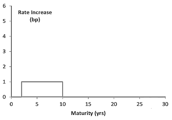
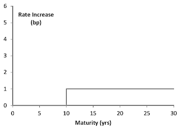
Forward Bucket Shifts

The bucketing procedure can be used for forward rates as well. Suppose the bucket rates as described in the previous section so that there are three buckets: 0–2 years, 2–10 years, and 10–30 years. Assume forward rates are calculated for six-month periods. Applying a one-basis-point shift to forward rates in the first bucket would involve increasing the forward rates for the six-month periods beginning in 0, 6, 12, and 18 months by one basis point. Similarly, applying a one-basis point shift to forward rates in the second bucket would involve increasing the forward rates for the six-month periods beginning in 24, 30, 36, 42, 48, and 54 months by one basis point. Applying a one-basis-point shift to forward rates in the third bucket would involve increasing the six-month forward rates starting in 60, 66, 72, …, months by one basis point. The decrease in portfolio value for a one-basis-point increase in all forward rates in a bucket is referred to as a forward bucket 01. The sum of these forward bucket 01s equals the DV01 calculated by changing forward rates.
Hedging using forward-rate, rate shifts is similar to the other hedging procedures that have been outlined earlier.

Spot rates can be calculated from forward rates. Suppose all rates are six-month rates expressed with semi-annual compounding. Let f_t be the forward rate for the period between t and t+ 0.5 years. The N-year spot rate (R) is then given by:

$(1 + 0.5R)^{2N} = (1 + 0.5f_0)(1 + 0.5f_{0.5})(1 + 0.5f_1) \dots (1 + 0.5f_{N-0.5})$

This formula can be used to calculate the impact of one-basis-point changes in forward rates on spot rates and therefore on the value of a portfolio or hedging instrument. Consider a simple portfolio consisting of a three-year bond with a face value of USD 100 and a coupon of 6% per year. Assume the term structure is flat at 4% with semiannual compounding.

Suppose there are three buckets: 0–1 years, 1–2 years, and 2–3 years.

a) When forward rates in the 0–1 year bucket are increased by one basis point, the value of the bond becomes

Suppose there are three buckets: 0–1 years, 1–2 years, and 2–3 years.

b) When forward rates in the 1–2 year bucket increase by one basis point, the value of the bond becomes

c) When forward rates in the 2–3 year bucket increase by one basis point, the value of the bond becomes

$\frac{3}{1.02} + \frac{3}{1.02^2} + \frac{3}{1.02^3} + \frac{3}{1.02^4} + \frac{3}{1.02^4 \times 1.02005} + \frac{3}{1.02^4 \times (1.02005)^2} = 105.5923$

These results are summarized in this table.

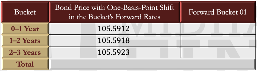
The total of the three forward bucket 01s

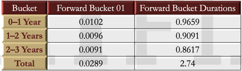
In the previous example, the forward rates in the first bucket have a larger effect on price than the forward rates in the second bucket, which in turn have a larger effect on forward rates than the forward rates in the third bucket. This illustrates a general phenomenon: The early forward rates affect more cash flows than the later forward rates, and therefore have higher 01s.
It is natural for swap traders to calculate their exposures to forward rates in the way described. Forward bucket 01s are also useful for contracts such as swaptions (i.e., options that enter a particular swap in the future).

Duration Measures

So far, we have considered how a DV01 (defined in terms of spot rates, par yields, or forward rates) can be decomposed in several measures that add up to the DV01. This can also be done with duration. It is known that

$Duration = \frac{10,000 \times DV01}{\text{Value of Portfolio}}$

Any of the 01 measures presented in this chapter can be converted into a duration measure using:

$Duration Measure = \frac{10,000 \times (01 Measure)}{\text{Value of Portfolio}}$

The forward bucket 01 measures in the previous table cane be converted to forward bucket duration measures. For example, the 0-1 year forward bucket duration is