Introduction

• Anticipating changes in the financial markets is an important component of risk management. Models play an important role in measuring and quantifying risks.
• There are two key theoretical models for market risk: modern portfolio theory (MPT) and the capital asset pricing model (CAPM).
• Market risk has attracted a great deal of academic research since the 1950s because of the abundance of available data on traded securities. As a result, market risk models have been empirically tested in various global markets.
• In risk models, there are several simplifying assumptions that allow them to deliver insights into the key factors and their interrelationships, without considering excess complexity. In this sense, a “good” financial model is one that helps to separate the major explanatory variables from the noisy background.
• Even a very simple model can be “successful” if it provides reasonably accurate forecasts and adds value to the decision-making process.
• Despite the criticism directed at risk management models following the 2007-2009 financial crisis—which saw models fail due to errors in selection, implementation, and over-interpretation—models and their underlying theories are still essential to modern risk management.
• While models are important tools, their implementation as well as the quality of the data and estimators used are also quite significant.

Modern Portfolio Theory

• Harry Markowitz demonstrated that a “rational investor” (i.e., an investor who is risk-averse and seeks to maximize utility) should evaluate potential portfolio allocations based upon the associated means and variances for the expected rate of return distributions. The theory also assumes

1. Capital markets are perfect, meaning that:
   • There are no taxes or transaction costs;
   • All traders have costless access to all available information; and perfect competition exists among all market participants
2. Returns are normally distributed – The assumption of normally distributed returns allows investor utility choices (as well as investment portfolios) to be stated simply in terms of the mean (i.e., performance) and variance (i.e., risk). With all else being equal, investors prefer a higher mean return and a lower variance.

• Investors seek to reduce the variance of their portfolio returns by diversifying their investments. Diversification is accomplished by investing in a portfolio of assets whose returns are uncorrelated. Specifically, diversification allows investors to offset specific risk exposures associated with individual assets.
• According to Markowitz, the level of investment in a particular financial asset should be based upon that asset’s contribution to the distribution of the portfolio’s overall return (as measured by the mean and variance). An asset’s performance is not judged in isolation, but rather in relationship to the performance of the other portfolio assets. In other words, what matters is the co-variability of the asset’s return with respect to the return of the overall portfolio.
• Theoretically, portfolio diversification enables the reduction of risk exposures to individual assets at zero cost. Therefore, investors should receive no compensation for taking on the specific risk (also known as the idiosyncratic risk) of any asset.
• Logically, a reduction in risk should result in lower expected returns. If the asset weights are appropriately selected, however, the resulting diversification can enable the optimization (i.e., maximization) of returns for any given level of risk.

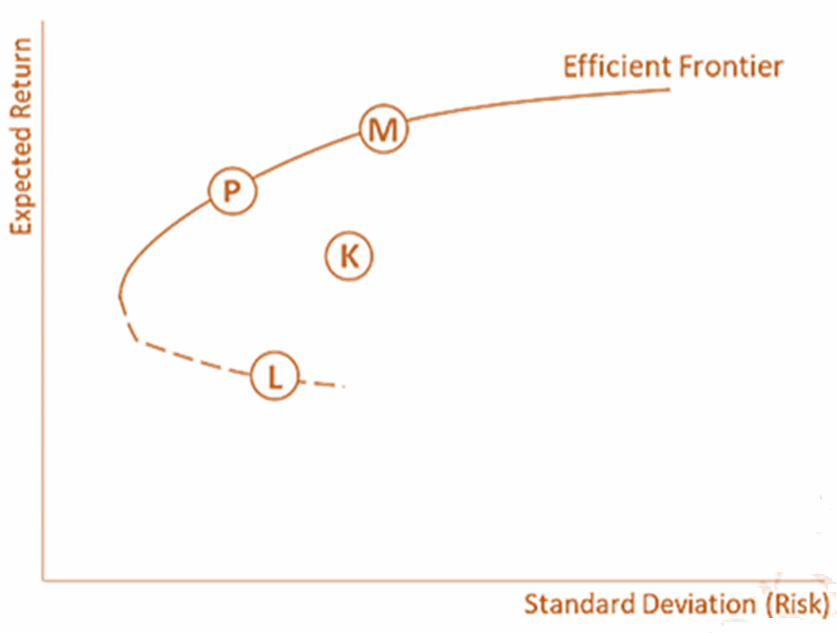
• Plotting the optimal returns for each level of risk results in the efficient frontier, which is represented by the curved solid line in this figure. Each point on this curve represents the portfolio of assets that is expected to offer the highest return for the given level of risk.
• In the previous figure, portfolio P offers the best return for any portfolio with the same level of risk. Meanwhile, portfolio K can be categorized as being suboptimal because there are portfolios that will offer better returns for the same level of risk (i.e., all the portfolios that lie vertically between portfolio K and the efficient frontier line).
• Along the efficient frontier, the only way to achieve a higher expected rate of return is by increasing the riskiness of the portfolio. Conversely, it is only by reducing the expected return that a less risky portfolio can be achieved.
• The dotted line in the plot represents the most inefficient portfolios (e.g., portfolio L) where the investor achieves the lowest expected return for each level of risk.
• This concept can be theoretically extended to the entire scope of investable assets. Portfolio M (called the market portfolio) assumes that the market achieves equilibrium and accordingly includes all of the risky assets in the economy weighted by their relative market values. In practice, stock market indices are used to represent the market portfolio.

• For the United States, a proxy for the market portfolio may be the S&P 500 index or the wider-based Russell 2000. Meanwhile, the FTSE 100 and the Euro Stoxx 50 are used for the U.K. and European markets (respectively).
• Diversification means that a security’s specific (i.e., idiosyncratic) risk should not be heavily (or at all) considered when it is being priced by the market.
• However, the role of diversification has been challenged in recent years. The average correlation of stock returns has increased from around 25% in the 1970s to between 30% and 40% in 2018.
• Correlations across asset classes have also increased substantially, even in normal market conditions. One commonly cited reason for this increase is the huge increase in basket trading via index-tracking mutual funds and exchange traded funds (ETFs). Through these vehicles, large baskets of assets composed of benchmark indices are traded simultaneously.

• Quantitative asset management techniques have been proposed to adapt to this new environment. These techniques consist of identifying risk regimes and optimizing portfolio allocations for each specific risk regime.
• If an asset manager anticipates a high-risk regime, she can switch her portfolio to a more conservative selection of investments. This may include an increased allocation toward low-risk assets, such as money market funds.
• Conversely, if a manager anticipates a low-risk regime, she can switch to a more aggressive asset allocation of equities, emerging markets, commodities, high yield bonds, and so on.

Each asset allocation is optimized to generate the highest return for the regime with which it is associated.

Capital Asset Pricing Model (CAPM)

• William Sharpe (1964) and John Lintner (1965) incorporated overall capital market equilibrium into the MPT theory. Specifically, Sharpe and Linter broke down the risk of an individual asset into specific risk (i.e., risk that can be diversified away) and systematic risk (i.e., risk that cannot be eliminated in the same manner). In their analyses, Sharpe and Lintner made several crucial assumptions, some of which they inherited from Markowitz’s MPT:
• Access to information for all market participants, meaning that all information is freely available and instantly absorbed
• No transaction costs, taxes, or other frictions
• Allocations can be made in an investment of any partial amount (i.e., perfect divisibility)
• All participants can borrow and lend at a common risk-free rate
• Any individual investor’s allocation decision cannot change the market prices

• The CAPM model shows that market equilibrium is achieved when all investors hold portfolios consisting of the riskless asset and the market portfolio. Each investor’s portfolio is just a combination of these two, with the proportional allocation between them being a function of the individual investor’s risk appetite.

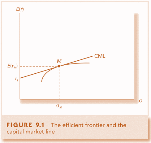
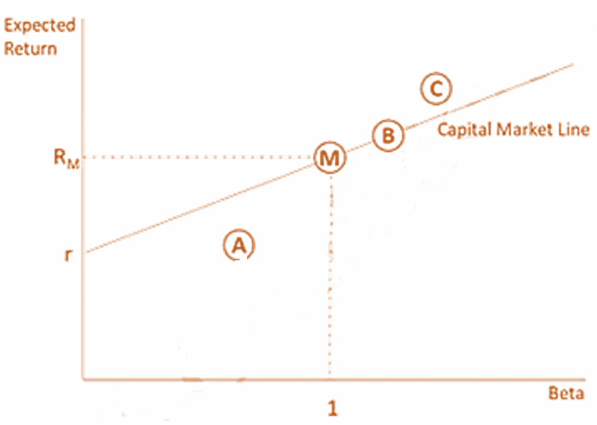
Capital Market Line

CAL becomes the CML if the optimal risky portfolio for all investors is the same which is the market portfolio.

Capital Market Line – Slope Interpretation Example

If you want to change the portfolio along the CML to another point such that increases by 1%, how much will be the increase in ? is the value of when when = 0

CAPM Beta

Accordingly, the expected return on a risky asset is determined by that asset’s relative contribution to the market portfolio’s total risk. This measure of systematic risk is named beta and is calculated as:
where and are (respectively) the returns on asset i and the market portfolio, and are their associated standard deviations. is the correlation between the returns on asset i and those on the market portfolio.

• The beta of the market portfolio is one by construction.
• From an investor’s perspective, beta represents the portion of an asset’s total risk that cannot be diversified away and for which investors will expect compensation. Hence, the higher the beta, the higher the risk (and therefore the higher the expected rate of return).

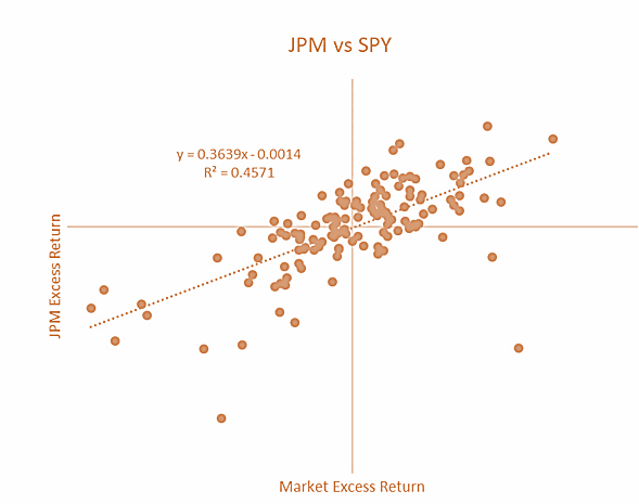
Beta – Estimation

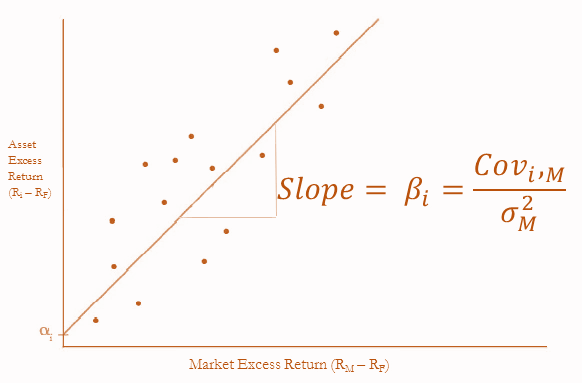
• Beta for an asset is estimated by regressing returns on the asset with market returns, where excess return on asset is taken as dependent variable and excess return on market index is taken as independent variable.
• Least square regression line is plotted. While plotting the linear fit of the points as closely as possible, the least-squares regression line is the one that has the smallest possible value for the sum of the squares of the distances of the points plotted from the line.
• The slope of this line is the estimate of beta which is given as

Beta – Estimation

• The regression line is known as security characteristic line.

CAPM Equation

• According to this model, the expected rate of return over a given holding period on a given asset i is
  

where

is the expected return of asset i over the holding period
is the rate of return on the risk-free asset.
is the market risk premium per unit of beta

is the expected return premium above the risk-free rate (as required by investors).

• The market risk premium is the difference between the expected rate of return of the market portfolio and the risk-free rate:
• This premium could be given by the difference between the rate of return on a broad market index (eg., the S&P 500) and a risk-free rate (e.g., the three-month U.S. Treasury Bill). In theory, should represent the expected return on portfolio of all risky assets in the market. In practice, however, a ‘broad enough’ index of traded shares is used as a proxy.

Deriving the CAPM – A Simple Approach

• The CAPM equation for the expected return on an asset can be derived in the terms of risk-free rate, beta and the excess market return over the risk-free rate.
• Idiosyncratic risk (or unsystematic risk or asset-specific risk) can be removed by diversification which is costless, and only systematic risk (or beta risk) is left.
• Diversification is costless and thus, investors should only be compensated for systematic risk (or beta risk), and portfolios with the same beta should have the same return.
• Expected return on an asset is a linear function of its beta.
• One point on this line is (0, ), as the risk-free asset lies on this line which has an asset beta of
• Another point on this line is the market portfolio which has a beta of 1. Hence, another point is (1, ).
• Putting these two in equation (1) we get
• a = and b = –

and hence the CAPM equation is

CAPM Example

• Consider the CAPM Equation :



The expected market return is 10% and the T-Bill rate is 4%. Find the expected return of a stock with : (a) = 1 (b) = 0 (c) = 0.6

Security Market Line

• The CAPM equation is represented by the security market line (SML).

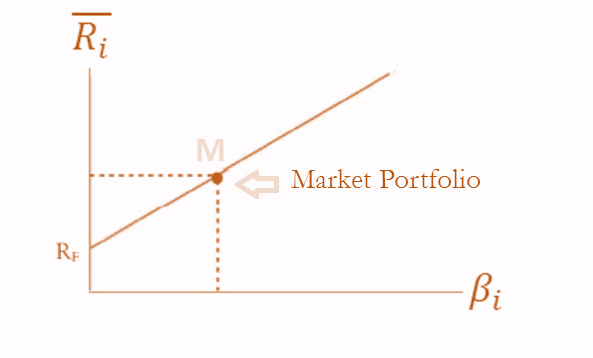
• If expected return is different than the expected return obtained from CAPM, then the asset is not correctly priced, and will not lie on the SML.
• An asset having an expected return which is lower than the CAPM return is overvalued, and it lies below the SML.
• An asset having an expected return which is higher than the CAPM return is undervalued, and it lies above the SML.

2020 Syllabus Variations

CAPM Application Example

CAPM Application

• Since its development, CAPM has become an important tool in understanding the behavior of prices in capital markets. Beta is also highly important to corporate managers focusing on creating shareholder value.
• Many corporations require a minimum return rate of return on the investment to assess the desirability of new ventures. This hurdle rate is often based on beta factor analyses, which are essentially how a firm understands the market’s expectations for its relative return (or how the market would view the relative return of the proposed venture/project). A failure to properly understand investor expectations can lead to a hurdle rate set at the wrong level. Note that a hurdle rate set too high can result in missed opportunities, whereas a rate set too low may result in sub-par investments. Either way, such errors can negatively impact beta-adjusted returns.
• The original CAPM was developed for discrete time intervals (e.g., one-year or one-month horizons). Subsequently, Merton (1972) extended the model to continuous time framework by assuming that trades are continuously executable and price changes are smooth (i.e., no jumps in prices).

Performance Measures Introduction

• In a world where the market is in equilibrium and is expected to remain in equilibrium, no investor can achieve an abnormal return (i.e., an expected return greater than that return predicted by the CAPM risk-return relationship). Each asset (or portfolio of assets) yields an identical rate of risk-adjusted return. So all securities will lie on the capital market line.
• Of course, this is not the case in the real world.
• First, it is not known exactly how expected values are determined. While they can be estimated, such estimations are always subject to measurement errors.
• Second, markets are rarely in equilibrium. And once they reach equilibrium, deviations from equilibrium are likely to occur almost instantaneously.

• In the real world, stocks and portfolios may yield a return in excess of, or below, the return with fair compensation for the risk exposure. This is the reason why portfolio managers rely on indices to measure the performance of a given stock or portfolio relative to the CAPM equilibrium risk-return relationship.

Treynor Measure

• The Treynor ratio (1965) is defined as :



Where
= expected return on the portfolio
= return on risk-free asset
= beta of the portfolio

• Treynor ratio is a measurement of the returns earned above the risk free rate, per unit of systematic risk.
• Comparing Treynor ratios of the given portfolio and the market portfolio tells whether portfolio risk is rewarded adequately or not.
• Treynor ratio is quite appropriate to compare the performance of well-diversified portfolios, as it only considers systematic risk.
• Treynor ratio is most appropriate for evaluating performance of a portfolio that only constitutes a part of the investor’s assets.
• Calculation of Treynor ratio requires a reference index to be chosen to estimate the beta of the portfolio.

Sharpe Measure

• The Sharpe ratio (1965, originally known as reward-to-variability ratio) is defined as :



Where
= expected return on the portfolio
= return on risk-free asset
= standard deviation of the expected returns

• Sharpe ratio is a measurement of the returns earned above the risk free rate, per unit of total risk.
• Sharpe ratio of the market portfolio is the slope of the CML.
• Comparing Sharpe ratios of the given portfolio and the market portfolio tells whether total risk taken is rewarded adequately or not.
• Sharpe ratio is quite appropriate to compare the performance of portfolios which are not very well diversified, as it also considers unsystematic risk along with systematic risk.
• Sharpe ratio is most appropriate for evaluating performance of a portfolio that constitutes an investor’s total investments.
• Calculation of Sharpe ratio does not require a reference index.
• The Treynor and Sharpe ratios will provide the same ranking for two assets that have identical correlations with the market.

Jensen’s Measure

• Jensen’s alpha is defined as :


Where
= expected return on the portfolio
= return on risk-free asset
= expected return on the market portfolio
= beta of the portfolio

• Jensen’s alpha is the portfolio’s excess return in excess of the return predicted by CAPM.
• Jensen’s alpha contains a benchmark, unlike Treynor and Sharpe measures.
• Jensen’s alpha is quite appropriate to compare the performance of portfolios within peer groups which are managed in a similar manner, and have quite comparable betas.
• The results obtained by Jensen’s measure depend on the choice of the reference index.
• Jensen’s alpha can become negative when managers follow a market timing strategy by varying the beta according to predicted market movements.

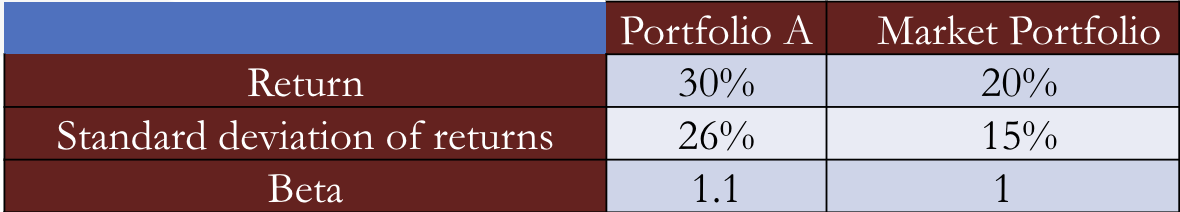
Example

• Given the following information about the performance data for Portfolio A and the Market Portfolio.

Relationships Between Measures

• Treynor and Jensen

• Sharpe and Jensen

• Sharpe and Treynor

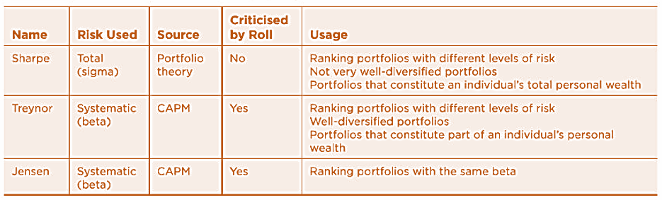
Characteristics of Measures

• The following table summarizes the characteristics of the three indicators

Extensions to Jensen Measure

• As Jensen’s alpha is excess return of some reference, it can be extended by replacing that reference with an appropriate value.
• If reference return is the required return on a portfolio A, which is based on CML, then



And the new alpha in this case will be

• Extensions of Jensen’s measure can also be done by using a reference return derived from a multifactor model or Black model.

Tracking Error

• Tracking error is the standard deviation of the difference in return between the portfolio and the benchmark, i.e.



Where

is the return on the benchmark portfolio

• Tracking error is used to assess success of the manager, and should be kept below a specified level by the manager by reallocating the portfolio regularly.
• It is necessary to find the right balance between frequency of reallocations and transaction costs, so that these costs do not impact the portfolio in a negative way overall.

Information Ratio

• The information ratio, or the appraisal ratio, is the residual return of the portfolio with respect to its residual risk, where the residual return is the excess return over the benchmark, and the residual risk is represented by tracking error, i.e.



• Information ratio is used to assess if the manager’s deviation from the benchmark has been rewarded with an adequate return or not.
• It is known as ‘information ratio’ because it makes an assessment of how well the manager has obtained and utilized information as compared to the average manager.

Sortino Ratio

• Sortino ratio is defined on the same lines as the Sharpe ratio. The risk free rate is replaced with a minimum acceptable return, denoted MAR, which is the return below which the investor does not want to fall. The standard deviation is replaced by semi standard deviation, denoted by SSD min which is the variability of only those returns that fall below MAR.

i.e.


Where


• Sortino ratio is more useful when returns are not symmetric. It differentiates harmful volatility from total volatility as it uses the portfolio’s standard deviation of only those returns which fall below the MAR, called downside deviation.

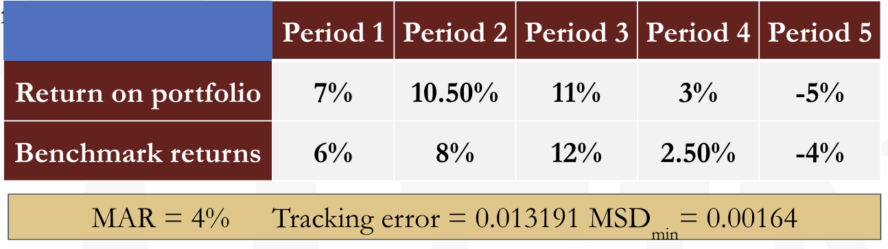
Example

• Given the following data: