Introduction

• The capital asset pricing model (CAPM) is a single-factor model that describes an asset’s expected rate of return as a linear function of the market’s risk premium above a risk-free rate. Beta is the coefficient (i.e., the slope) of this relationship.
• The Arbitrage Pricing Theory (APT) is based on the reasoning behind CAPM. However, it explains an asset’s expected rate of return as a linear function of several market factors.

The Arbitrage Pricing Theory

• APT suggests that multiple factors can help explain the expected rate of return on a risky asset. These factors may include indices on stocks, bonds, and commodities, as well as macroeconomic factors. However, the model does not say which of these factors adds to the explanatory power of the relationship.
• APT was initially proposed in 1976 by Professor Steve Ross. Unlike CAPM, APT does not assume investors hold efficient portfolios (as defined within the mean-variance framework) and does not assume risk aversion. Instead, APT has three underlying assumptions.
  • Asset returns can be explained by systemic factors.
  • By using diversification, investors can eliminate specific risk from their portfolios.
  • There are no arbitrage opportunities among well-diversified portfolios. If any arbitrage opportunities were to exist, investors would exploit them away.

  According to APT, the return on a security is given by:

  

  where:

  is the rate of return on security ( = 1,2, …, N) with expected return E (Ri);

  is the difference between the observed and expected values in factor k (it is also known as the surprise factor);

  is a coefficient measuring the effect of changes in factor Ik on the rate of return of security i; and

  is the noise factor (i.e., the idiosyncratic factor).

• APT was later tested and it was found that the following set of macroeconomic factors were important in explaining the realized average rates of return on stocks traded on the New York Stock Exchange (NYSE):
  • The spread between long-term and short-term interest rates (reflecting shifts in time preferences);
  • Expected and unexpected inflation;
  • Industrial production (reflecting changes in cash flow expectations); and
  • The spread between high-risk and low-risk corporate bond yields (reflecting changes in risk preferences).

• It noted that well-diversified portfolios are volatile, and that the volatility of a long portfolio is approximately half of the average volatility of its constituent assets. It was concluded that this was indicative of systematic risk drivers that limit the effects of diversification within an asset class. Without these risk drivers, a diversified portfolio would have much smaller volatility.
• It was also noted that well-diversified portfolios exhibit high correlations when constrained to the same asset class, whereas there is much less correlation when portfolios are diversified across multiple asset classes. This suggests the existence of multiple systematic factors (otherwise there would be higher correlations across various asset classes/countries/sectors).
• The basic premise of APT is that investors can create a zero-beta portfolio with zero net investment. If such a portfolio yields a positive return, however, then a sure profit can be realized through arbitrage. The fundamental result is that the absence of arbitrage opportunities requires the expected return on all well-diversified portfolios to satisfy



where

is the return on a well-diversified portfolio with expected return ;

is the factor loading for the portfolio P related to factor k;

is the expected rate of return on the zero-beta portfolio (i.e., the risk-free rate) such that

for = 1, … ,K; and

– is the risk premium associated with factor

• APT and CAPM refer to the expected rate of return on security i. However, because the expected rate of return is unobservable, one must use the realized historical average instead.
• CAPM is a special case of the APT approach.
  • CAPM is a one-factor model and thus the market index is the only variable used to explain the expected return for any security.
  • The APT is a multi-factor model where several different indices can be used to explain the variation in expected rates of return. APT is often used to decompose the factors’ respective contributions to the expected return.

• An additional benefit of the APT approach (as well as all factor approaches) lies in how they help facilitate risk analyses.

Multifactor Models of Risk and Return

• Empirical studies of the single-factor market model (i.e., CAPM) show that its explanatory power is rather low. Additional studies indicate the existence of other factors related to firm attributes including size, financial ratios (P/E, cashflow/price, and debt/equity), revenue trends, and historical returns-that are also correlated to average rates of return.
• Fama and French (1996) presented a three-factor model that captures these factors. Their model extends CAPM by adding two additional factors:
  • Small Minus Big (SMB) (i.e., the difference between returns from small stocks and those from large stocks)
  • High Minus Low (HML) (i.e., the difference between the returns on stocks with high book-to-market values and those of stocks that have low book-to-market values)

• The three-factor model proposed by Fama and French is then: where

is the expected return on portfolio P;

is the risk-free interest rate;

is the excess return on the asset, which is governed by the impact of management. In equilibrium, = 0; and

– is the expected premium corresponding to market factor

E(SMB) is the expected premium corresponding to size factor

E(HML) is the expected premium corresponding to value factor

• According to Fama and French,
  • The slope of HML is a proxy for relative distress: Strong (weak) firms with consistently high (low) earnings have negative (positive) HML slopes.
  • The SMB factor captures the covariation in returns on small stocks (i.e., the small firm effect).
• Fama and French extended the model in 2015 by suggesting two additional factors:
  • Robust Minus Weak (RMW), which is the difference between the returns of companies with high (robust) and low (weak) operating profitability, and
  • Conservative Minus Aggressive (CMA), which is the difference between the returns of companies that invest conservatively and those that invest aggressively.

Adding these two factors, Fama and French showed that the HML factor is redundant. Other versions of this model (e.g., Carhart (1997)) include a momentum factor (MOM), which is the difference between stocks that have risen in value over the prior month (i.e., winners) versus those that have fallen in value (i.e., losers).

Example

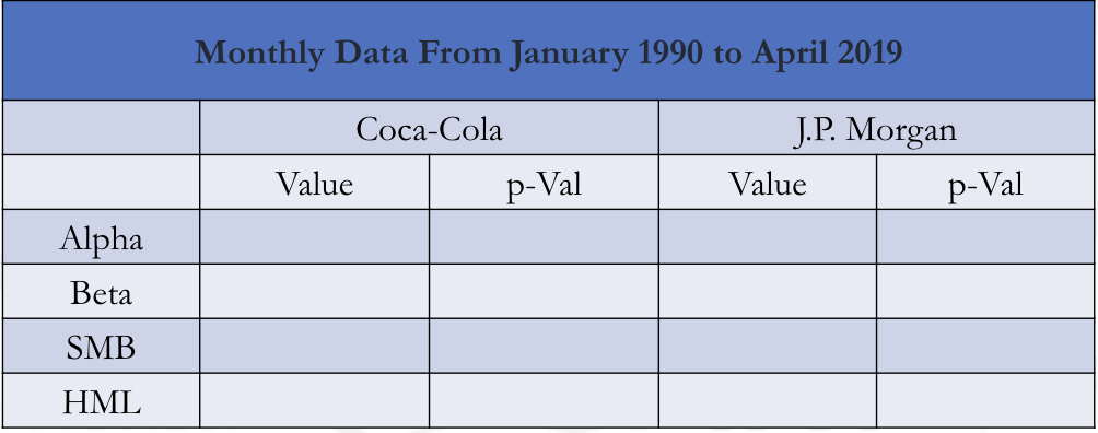
• Consider two companies: Coca-Cola and J.P. Morgan. Using monthly returns from January 2011 through April 2019, the three-factor Fama-French coefficients are estimated in this figure.

• An analyst believes that a company’s Fama- French dependencies are:



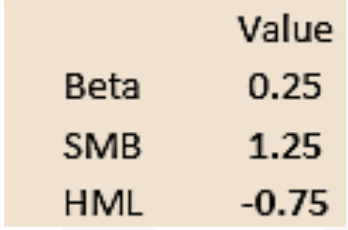
The analyst believes that the firm can generate an extra 3.0% return annually because it has an advantage over its competitors. The market forecast is

• A 12.5% return on equities over the next year;
• An SMB of 3.5%;
• An HML of 0.0%; and
• A risk-free rate of 1.5%

The expected return for the company would be

Example –

• State Street Global Advisors has formulated several tradable baskets of equities, made from subsets of the S&P 500, that are designed to track specific indices. These equities are part of the Standard and Poor’s Depository Receipts (SPDR) Exchange Traded Fund (ETF) family and can be traded in the same way as regular equities.

These tradable ETFs can be used in an explanatory multi-factor return model (in the same way as CAPM uses a broad market index or Fama-French relies upon the broad market and two relative return indices)

The nine sector SDPRs are in the following table.

Symbol	Sector
XLB	Materials
XLE	Energy
XLF	Financials
XLI	Industrials
XLK	Technology
XLP	Consumer Staples
XLU	Utilities
XLV	Health Care
XLY	Consumer Discretionary

Factor Hedging

• While idiosyncratic (i.e., specific) risk can theoretically be eliminated through diversification, the same is not true for systematic risk. However, factor betas can be used to construct a hedging strategy to eliminate systematic risk.
• Each factor can be regarded as a fundamental security and can therefore be used to hedge the same factor that is reflected in a given security.
  • If the goal is to hedge out all the factor risks and create a zero-beta portfolio, then an opposite position can be taken in each of the factors so that the combined portfolio contains no factor exposures.
  • If the goal is to leave a portfolio exposed to certain types of systematic risks, then not all factor exposures need to be neutralized.
• The selection of the appropriate systematic factors depends (in part) on judgment and there is no single perfect set of factors for all investors, based on their risk-adjusted return objectives.

PS – Also watch 2019 Video – Factor Portfolios section in this same chapter.

Challenges in Hedging Exposure

• There is a tradeoff between the cost of hedging and the need to keep the hedge aligned to the portfolio. If the hedging strategy is not implemented on a continuous basis, then tracking errors will appear. If the hedging strategy is updated too frequently, trading costs will be high and drag down overall performance.
• Another challenge is model risk, which includes both factor model error and the potential for errors in implementation. Factor model errors occur when a model contains mathematical errors or is based on misleading/ inappropriate assumptions.
  • For example, a hedging strategy that is based on linear factor models that fail to capture nonlinear relationships among the factors will be flawed.
  • Another common error in model building is to assume stationarity in the underlying asset distribution, as often such distributions can evolve over time.
  • Additionally, assumptions built into models may fail to hold in certain conditions, such as during stressed markets. During the 2007-2009 financial crisis, for example, many market-neutral hedge funds performed poorly.