Introduction

• Derivatives traders must manage the risks they take. The Greek letters (or Greeks, as they are sometimes called) are designed to provide information about these risks. Some Greek letters are concerned with movements in the price of the underlying asset; some are concerned with volatility changes; and others involve interest rates and dividend yields.

• Typically, a trader is subject to limits on how large the Greek letters can be. If one of the Greek letters exceeds the applicable limit near the end of the trading day, a trader must either execute a trade that corrects the situation or seek special permission from the risk management function to maintain the existing position.

Introduction – Managing Derivatives Risk

• Suppose a trader has sold a client over-the-counter European call options contract to buy one million shares of a stock. The stock price is USD 100 per share, and the strike price is USD 105. The risk-free rate is 4% per annum, the volatility of the stock price is 25%, and the time to maturity is one year. The Black-Scholes-Merton pricing equation shows that the theoretical price of such an option is USD 9.56.

• Suppose the price obtained by the trader for one million call options is USD 10 million. The theoretical value of the transaction (USD) to the trader is

10,000,000 – 9,560,000 = 440,000

• Three choices to manage the risk of the above position are:

1. Buy one million options that are the same as those sold
2. Do nothing
3. Cover the position by buying one million shares.

• The first strategy would provide a perfect hedge. However, it is unlikely to be financially attractive.
• The second strategy (sometimes referred to as a naked position) works well if the stock price stays below USD 105 for the next year. But it can lead to heavy losses when the stock price increases heavily (which is definitely possible with a 25% volatility).
• The third strategy works well if the option is exercised. However, there is the potential for a considerable loss if the price declines.

Stop – Loss Strategy

• Another possible hedging strategy is called the stop-loss strategy. This is a mixture of the second and third strategies just considered. Under this approach, the trader attempts to have a naked position when the option is out-of-the-money (i.e., the stock price is less than the strike price) and a fully covered position when it is in-the money (i.e., the stock price is greater than the strike price). In the previous example, when the price of the stock is below USD 105, the trader maintains a naked position. As soon as the price rises above USD 105, the trader covers the position by buying one million shares. If the price subsequently falls below 105, the trader sells the shares. If it later rises above USD 105, the trader repurchases the shares.
• If it is assumed the stock can be bought at USD 105 as it moves in-the-money and that it can be sold at USD 105 as it moves out-of-the-money, the stop-loss strategy leads to one of the following results.
  • If at the end of the year the stock price is less than USD 105, the trader has a naked position and makes a USD 10 million profit.
  • If at the end of the year the stock price is more than USD 105, the trader has a fully covered position. Again, the trader makes a net profit of USD 10 million.
• This strategy also appears to work well if the option is initially in-the-money. The trader must initially cover the position and then makes a profit corresponding to the difference between the price at which the option is sold and its initial intrinsic value.
• Unfortunately for option traders, the stop-loss strategy is flawed. When the stock price reaches USD 105, the trader does not know whether the next price move will be up (so that the option moves in-the-money) or down (so that the option moves out-of-the money). If the stock price moves from USD 104.9 to USD 105 and the trader buys one million shares, it is possible that the next price move will be back to USD 104.9. Similarly, if the stock price moves down from USD 105.1 to USD 105, and the trader sells one million shares, the next price move might be back up to 105.1
• If the stock price never reaches the strike price of USD 105, the stop-loss strategy works well. If it passes through the strike price level of USD 105 just once, the strategy still works well. But if it passes through the strike price level many times, the strategy could be very expensive.
• Whatever the hedging strategy used (and if the Black-Scholes-Merton assumptions hold), the present value of the expected cost of hedging should always be the Black-Scholes-Merton value (USD 9.56 million in the previous example). In a good hedging strategy, the cost of writing and hedging the options is always close to this expected cost. In the previous example, this would lead to a profit of close to USD 440,000 (= 10 million – 9.56 million) regardless of the direction of movement of the stock price over the next year.
• The stop-loss strategy is not a good hedging strategy because the cost is sometimes much more than the theoretical price of the option.

Delta Hedging

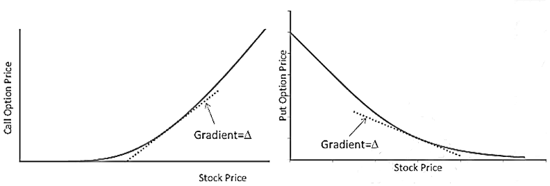
• Delta of a derivative is the rate of change of the price of the derivative with respect to the change in the price of the underlying asset. The formula for the delta of a derivative dependent on a stock price S is

• Where δS  is a small change in the stock price, and δf is the resultant change in the value of the derivative (with everything except the stock price being kept fixed). Deltas for call and put options are illustrated in this figure

• The delta of a long position in a European call option on a non-dividend paying stock is

• The delta a long position in a European put option on a non-dividend-paying stock is

• The parameter d_1 is defined (as in the Black-Scholes-Merton equations) as:

where K is the strike price, T is the time to maturity, and r is the risk-free rate for maturity T. By convention, the volatility σ is set equal to the option’s implied volatility (rather than a historical estimate of volatility) when all Greek letters are calculated. The function N is the cumulative normal distribution function for a standard normal variable with mean zero and standard deviation one.

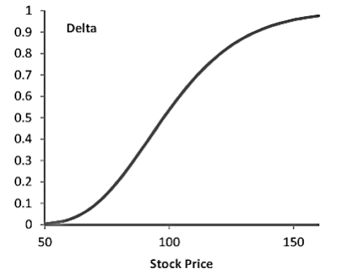
Call Delta

• The delta of a long position in a call option is positive since the price of a call option increases as the stock price increases. This figure shows the variation of delta for a call option with respect to the variation in the stock price.

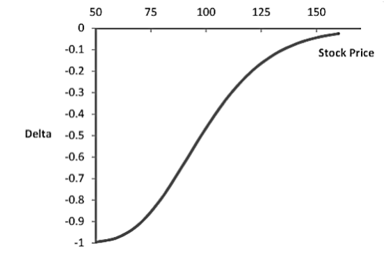
Put Delta

• The delta of a long position in a put option is negative because the price of a put option decreases as the stock price increases. This figure shows the variation of delta for a put option with respect to the variation in the stock price.

Delta Hedging

• Let’s consider again the European call option from the previous example where the stock price is USD 100, the strike price is USD 105, the risk-free rate is 4%, the volatility is 25%, and the time to maturity is one year. In this case:

The trader who has sold one million options (i.e., has a short position in one million options) has a delta of:

To hedge the position, he or she should ______________________ shares. The gain (or loss) on the option will then be offset by the loss (or gain) on the shares. Suppose the stock price increases by USD ____ , the option price is expected to increase by about ____________________.

The loss on the short option position will be _______________________________

The gain on the __________________ shares will be _______________________

so that the net gain/loss is ____________________.

• One problem for the trader is that delta does not remain constant. Delta hedging is therefore not a “hedge and forget” strategy. The hedge must be adjusted every day (or even more frequently). Adjustments to the hedge are referred to as rebalancing.

• Suppose that after one day the stock price rises to USD 100.4. The option now has ________ days to maturity and the new delta is

• The delta of the trader’s position is now:

_________________________________________________

so that the number of shares that must be bought for the hedge is now _________________

The trader must therefore buy an additional _____________________________ shares

•Suppose that the stock price falls to USD 99.9 by the end of the next day. The time to maturity is now _____________________ days and the new delta is

______________________________________________

To rebalance the hedge, the trader must sell ______________________________ shares to bring the holding down to _____________________________ shares.

• Delta hedging continues in this way until the option expires.

Vega

• In practice, volatility changes through time, and this increases the risk for derivatives traders.

• Consider the options trader in the previous section. Suppose that while the stock price stays at USD 100 during the first day of the option’s life, the volatility increases from 25% to 28%. The trader’s position would then decline in value since the options sold have increased in value.

• Vega is the Greek letter that measures the trader’s exposure to volatility. It is defined as:

where δσ is a small change in volatility (with everything else remaining the same), and δf is the resultant change in the value of the derivative. The volatility σ is actually the implied volatility.

• A long position in either a call option or a put option has a positive vega. The vega of a European call (or put) option on a non-dividend paying stock is given by:

Here N′(x) is the standard normal probability density function:

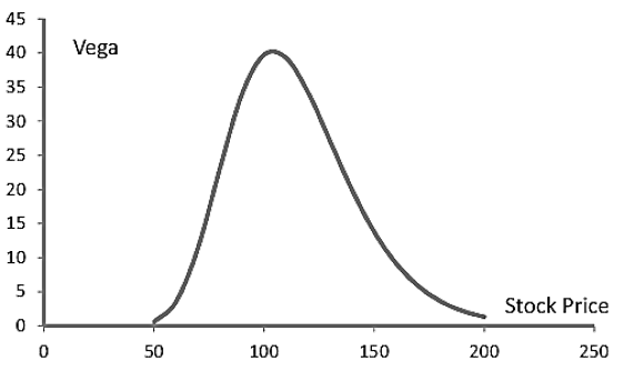
• Vega is greatest for options that are close-to-the-money (i.e., options where the stock price is close to the strike price). Vega tends to zero as the option moves deep-out-of-the-money or deep-in-the-money. When an option is deep out-of-the-money, it almost certainly will not be exercised regardless of volatility changes; when it is deep-in-the-money, it will almost certainly be exercised regardless of volatility changes.

• This figure show the variation of vega of an option with a stock price for a call or put option with a strike price of 105 and a time to maturity of one year when the risk-free rate is 4% and the volatility is 25%.

• Consider again a call option on a stock worth USD 100 when the strike price is USD 105, the risk-free rate is 4%, the volatility is 25%, and the time to maturity is one year.

This means that the vega of a long position in one option is

______________________________________________

In the formula for vega, it is assumed that volatility is expressed as a decimal. The change in the price of the option for a 0.01 (1%) change in volatility is ______________________________

The change in the value of a portfolio that has sold options on one million shares is __________________________________________ per 1% increase in volatility.

• Note that the vega suggests that a 3% increase in volatility (e.g., from 25% to 28%) leads to a loss of __________________________________________.

This is approximately the same as the ______________________________ million loss which was calculated earlier by substituting a volatility of 28% for 25% into the Black-Scholes-Merton model. This illustrates that the value of an option is approximately linear in volatility.

• Calculating vega from the Black-Scholes-Merton model may seem strange since the model assumes that volatility is constant. Indeed, models have been developed where the volatility changes in an uncertain way over time. However, the vega calculated from these models is similar to the Black-Scholes-Merton vega.
• Unfortunately, hedging vega risk is not as easy as hedging delta risk. The vega of a position in the underlying asset is zero. This means that trading the underlying asset does not affect the vega of a portfolio of derivatives dependent on the asset. Vega can only be adjusted by taking a position in another derivative dependent on the same asset.
• Suppose a delta-neutral portfolio dependent on an asset price has a vega of ______________.
• An option on the same asset can be traded that has a delta of _____________ and a vega of _________________. To hedge, number of options needed can be calculated by solving
• However, an amount of delta equal to  ____________________ is introduced into the portfolio. The trader must therefore short _________________ shares to maintain delta neutrality.

Gamma

• The gamma of a stock price–dependent derivative measures the sensitivity of its delta to the stock price. It is defined as:

where δS is a small change in the stock price, and δ(Δ)  is the resultant change in delta.

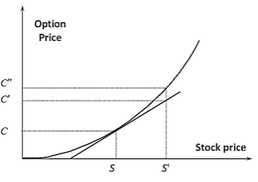
• Delta hedging assumes the relationship between the option price and the stock price is linear; it is actually non-linear. Gamma is a measure of the error made by this linearity assumption.

• Consider this figure. When the stock price moves from S to S’, delta hedging assumes the option price will move from C to C’; in fact, it moves from C to C’’.
• The risk associated with stock price movements then depends on how much the stock price could change over one day, and how much curvature there is in the relationship between the option price and the stock price. Gamma measures this curvature. For a delta-neutral portfolio, gamma measures the risk associated with relatively large changes in stock price between hedge rebalancing. Small stock price changes do not create a lot of risk since the relationship between the option price and the stock price is approximately linear for small changes.

• Gamma is positive for a long position in either a call option or put option. The gamma of a call (or put) option on a non-dividend paying stock is

• One important difference between gamma and vega is that while vega increases as the time to maturity increases, gamma decreases.

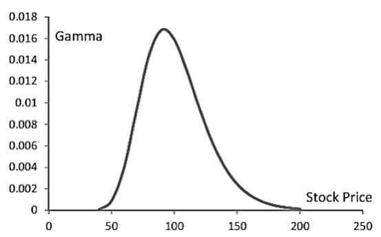
• This figure show the variation of gamma of an option with a stock price for a call or put option with a strike price of 105 and a time to maturity of one year when the risk-free rate is 4% and the volatility is 25%. Gamma is similar to vega in that it is greatest for options that are close-to-the-money and approaches zero as the option moves deep-in-the-money or deep-out-of-the money.

• Consider the same  call option on a stock with a price of USD 100 when the strike price is USD 105, the time to maturity is one year, the risk-free rate is 4%, and the volatility is 25%.

This means delta changes by  _____________ per unit change in the stock price.

• Gamma (like vega) can be changed only by taking a position in a derivative. This is because the position in the underlying asset has zero gamma. The procedure for making gamma zero (by trading another option) is similar to that given earlier for making vega zero.
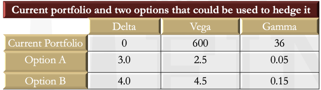
• Suppose the requirement is to make both gamma and vega zero. In theory, this can be done with two options. Consider the parameters of the portfolio and the available options as indicated in this table

Theta

• The theta of an option is the rate of change in its value over time. When time is measured in years, the theta of long positions in European call options and put options are

• Consider again the same European call option where the stock price is USD 100, the strike price is USD 105, the risk-free rate is 4%, the volatility is 25%, and the time to maturity is one year. The theta of the option is

__________________________________________________________

This means that if nothing changes, a long position in the option loses money at the rate of _________________________ per year

• Theta is usually negative for a long option position because (with all else remaining constant) options lose value as time passes. Theta differs from the other Greek letters in that there is no uncertainty about the passage of time (whereas there is uncertainty about a stock’s price or its volatility). As a result, traders can accurately estimate what will happen to an option price if one day passes with no other changes.
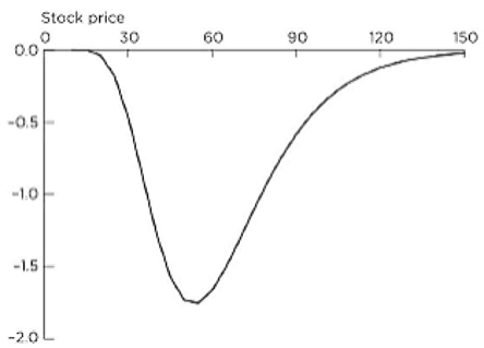
• This figure show the variation of theta of an option with a stock price for a call or put option with a strike price of 50 and a time to maturity of two years when the risk-free rate is 0% and the volatility is 25%.
• When theta is highly negative, gamma tends to be highly positive; when theta is highly positive, gamma tends to be highly negative.

Rho

• The rho of an option measures its sensitivity to interest rates.

• When interest rates are expressed as decimals, the formulas for the rho of a European call and put option on a non-dividend paying stock are

• Interest rate uncertainty is usually not as important for an option book as the uncertainty surrounding the asset price or its volatility.

• Consider again the same European call option where the stock price is USD 100, the strike price is USD 105, the risk-free rate is 4%, the volatility is 25%, and the time to maturity is one year. The rho of the option is

• This means that a 10-basis point (0.1%) increase in the interest rate (with nothing else changing) can be expected to increase the option price by ______________________

Portfolios With Example

• Any of the Greek letters for a portfolio of derivatives dependent on the same asset can be calculated as the weighted sum of the Greek letters for each portfolio component. For example, if a portfolio consists of the following items.
  • A long position in 50,000 call options where the delta, vega, and gamma of each option are 0.46, 3.3, and 0.13 (respectively).
  • A short position in 20,000 call options where the delta, vega, and gamma of each option are 0.33, 4.2, and 0.15 (respectively).
  • A short position in 30,000 put options where the delta, vega, and gamma of each option are -0.54, 3.0, and 0.08 (respectively).
• For the portfolio, the delta, vega, and gamma are

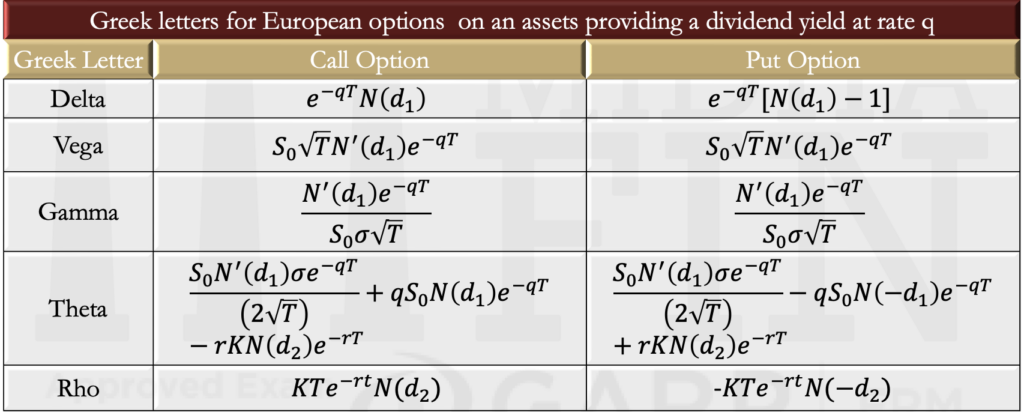
Other European Options

• The previous formulas are adjusted when there is a dividend yield at rate q.
  • For options on stock indices, q is set equal to the dividend yield on the index.
  • For options on currencies, q is set equal to the foreign risk-free rate.
  • For options on futures,  q is set equal to r.
  • An exception is the formula for the rho of a European futures option; this is –fT, where f is the price of the option.
• The formulas for are adjusted to:

Portfolio Insurance

• Asset managers are sometimes interested in acquiring a put option on their portfolio to provide protection against a market decline. They can create the option synthetically by imagining they are hedging a short position in the put option. Instead of taking a position in the underlying asset that neutralizes the delta of an existing option, they match the delta of the option they are trying to create.
• Suppose a portfolio is worth USD 100 million and that the asset manager wants to provide protection against the value falling below USD 90 million during the next six  months. The portfolio has a volatility of 25%, the risk-free rate is 3%, and the dividend yield is 2%. The manager therefore wants to create a put option where , K=90 million, r=0.03, q=0.02, σ=0.25, and T=0.5.

The delta of the option is In this case:

And the delta is

To match deltas, the asset manager should therefore sell ____________ of the portfolio. As time passes, delta changes.

• If the portfolio mirrors an index, the portfolio manager can keep the portfolio intact and buy options on index futures on an exchange. If the options market is not liquid enough to accommodate the manager’s desired trade, the required options on index futures can be created synthetically by trading the futures contracts themselves in the way we have described.
• Portfolio insurance was popular up until the late 1980s. However, its weaknesses were exposed when the Dow Jones Industrial Average dropped by more than 20% over a single day (this was Monday, October 19, 1987, and it is commonly referred to as Black Monday).
• When the market started to drop, portfolio insurers sent sell orders to the exchange. This, in turn, made the market drop even further. As a result, there were more sell orders from portfolio insurers. The volume of sell orders overloaded the stock exchanges, and trades could not be handled immediately. As a result, portfolio insurance proved less effective than predicted. Unsurprisingly, it has become much less popular since 1987.