What is the Black-Scholes model ?

The Black-Scholes model is used to price European options on non-dividend paying stocks.

How does the Black-Scholes model assume stock price movements ?

It assumes stock returns are normally distributed over short periods, leading to lognormal distribution over longer periods.

What is implied volatility ?

Implied volatility is the market's forecast of a stock's volatility, inferred from the prices of options.

What is the difference between European and American options ?

European options can only be exercised at expiration, while American options can be exercised anytime before expiration.

What is a volatility smile ?

A volatility smile is a pattern where implied volatility is low for at-the-money options and higher for in/out-of-the-money options.

How is delta used in options trading ?

Delta measures the sensitivity of an option's price to changes in the price of the underlying asset.

What is the significance of the lognormal distribution in the Black-Scholes model ?

The lognormal distribution ensures that stock prices remain positive and reflects realistic price movements over time.

How does the Black-Scholes model handle dividends ?

For dividend-paying stocks, the model is adjusted by subtracting the present value of expected dividends from the stock price.

What is put-call parity ?

Put-call parity is a relationship between the prices of European call and put options with the same strike price and expiration.

How are options on futures priced ?

Options on futures are priced using Black’s model, which adjusts for the specific behavior of futures contracts.

The Black-Scholes-Merton Model

Introduction

The Black Scholes pricing formula applies to European options on non-dividend paying stocks. It can be extended to European options on stocks paying discrete dividends and to European options on other assets (such as stock indices, currencies, and futures). It does not apply to American options, which must be valued using the binomial tree methodology explained in the previous chapter.

Stock Price Movements

The Black-Scholes-Merton model assumes that the return from a non-dividend paying stock over a short period of time is normally distributed.
If μ is the mean return and σ is the volatility, then the return in time ∆t is assumed to be normal with mean μ∆t and standard deviation $\sigma\sqrt{\Delta t}$ .
Theoretically, this is true only when ∆t tends to zero.
Practically, it is approximately true for a small ∆t.

EXAMPLE –

Let a stock whose price is USD 100, has an annual mean return (μ) is 12% per year, and an annual volatility of 25% per year. The probability distribution for the stock’s return over one week is approximately normal.

THE LOGNORMAL DISTRIBUTION

When the return on a stock over a short period is normally distributed, the stock price at the end of a relatively long period has a lognormal distribution. This means the logarithm of the stock price (and not the stock price itself) is normally distributed.

The key differences are between a normal and a lognormal distribution are as follows:

A normal distribution is symmetrical and the variable can take any value from negative infinity to infinity.

A lognormal distribution is skewed and the variable can take any positive value.

Since the future stock price cannot be negative, the resulting model with lognormal distribution for future stock prices is consistent with this observation.

The standard deviation of the change in the stock price S in time ∆t is Sσ√Δt. This standard deviation decreases with a decrease in stock price, Hence, movements in the stock price become smaller, and thus the stock price cannot become negative.
Let be the stock price at time zero and S_T as the stock price at time T. It can be shown that:
- The expected value of S_T is given by: $E(S_T) = S_0 e^{\mu T}$
- The expected value of the logarithm of the stock price at time T is $E(\ln(S_T)) = \ln(S_0) + (\mu - \frac{\sigma^2}{2})T$
- The standard deviation of the logarithm of the stock price is $SD(\ln(S_T)) = \sigma \sqrt{T}$
- The expected value of S_T is given by: $E(S_T) = S_0 e^{\mu T}$
- The expected value of the logarithm of the stock price at time T is $E(\ln(S_T)) = \ln(S_0) + (\mu - \frac{\sigma^2}{2})T$
- The standard deviation of the logarithm of the stock price is $SD(\ln(S_T)) = \sigma \sqrt{T}$

Since ln⁡ is a non-linear function, the mean of the stock price’s logarithm is not the logarithm of the mean stock price, i.e.

$E(\ln(S_T)) \neq \ln(E(S_T))$

In the earlier example, where the stock had a price of USD 100, annual mean return of 12%, and annual volatility of 25%. To construct a confidence interval for the stock price at the end of two years, expected mean and standard deviation of the logarithm of the stock price at that time are required.

Return Calculations

The realized return R from the stock in time T (when measured with continuous compounding) is given by:

$S_T = S_0 e^{RT}$

so that

$R = \frac{1}{T} \ln\left(\frac{S_T}{S_0}\right)$

This is normally distributed with mean:

$\mu - \frac{\sigma^2}{2}$

and standard deviation:

$\frac{\sigma}{\sqrt{T}}$

In the model, it has been assumed that the expected return over a very short period (theoretically, an infinitesimally short period) is μ. However, the return over a finite time period of length T is $\mu - \frac{\sigma^2}{2}$ . Although, these results seem inconsistent, but they are, in fact, consistent as that the return in time T is not the arithmetic average of the returns over n short periods of length ∆t.
To illustrate this, suppose USD 100 is invested for three months and the returns per month (with monthly compounding) are 4%, 10%, and -8%.
Similarly, if the length of each period (one month in our example) is made progressively smaller, then the expected return over time T with continuous compounding is $\mu - \frac{\sigma^2}{2}$ , and the expected return over an infinitesimally short period. is μ. Clearly $\mu - \frac{\sigma^2}{2} < \mu$

Volatility

Volatility (denoted by σ) is a measure of the uncertainty about the returns provided by an investment. It can be defined as the annualized standard deviation of the return (measured with continuous compounding). Risk managers often approximate volatility per day as the square root of the average squared daily return. This approximation works reasonably well for daily data. A more precise estimate can be obtained, which is shown here.

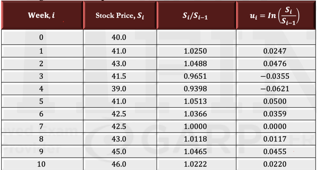
Consider a data set on the price of an asset (e.g., a stock) at intervals of τ years (e.g., for monthly data, τ = 1/12; for weekly data, τ= 1/52). If S_i is the i^th observation (0 ≤ i ≤ n), then the continuously compounded return between times i-1 and i is

$u_i = \ln\left(\frac{S_i}{S_{i-1}}\right)$ i=1,2,…,n

Let s be the standard deviation of u_i. An estimate of the volatility per year is

$\frac{s}{\sqrt{\Delta t}}$

Consider the weekly observations on a stock price in the second column of this table. The price relatives (i.e., the price in the current week divided by the price in the previous week) are in the third column. The logarithm of the price relative is shown in the fourth column.

Measuring Time

When volatility is calculated and options are valued, time is measured in trading days (i.e., days when the market is open), and not the actual number of days.

There are usually assumed to be 252 trading days in a year so that:

$Annual Volatility = Daily Volatility \times \sqrt{252}$

The life of an option is calculated in trading days. For example, if there are 56 trading days to maturity, the life is calculated as 0.222 (= 56/252) years.

Assumptions

The assumptions necessary to derive the Black-Scholes-Merton options pricing model are as follows:
- The behavior of stock prices corresponds to the lognormal model discussed earlier with μ and σ held constant.
- There are no transaction costs or taxes and all securities are perfectly divisible.
- There are no dividends on the stock during the life of the option.
- There are no riskless arbitrage opportunities.
- Security trading is continuous.
- Investors can borrow or lend at the same risk-free rate, which is constant through time.
- The options being considered cannot be exercised early.
Some of these assumptions have been relaxed in subsequent research. For example, r and σ can be functions of time, and some results can be extended for situations where dividends are anticipated.

No-Arbitrage For Options

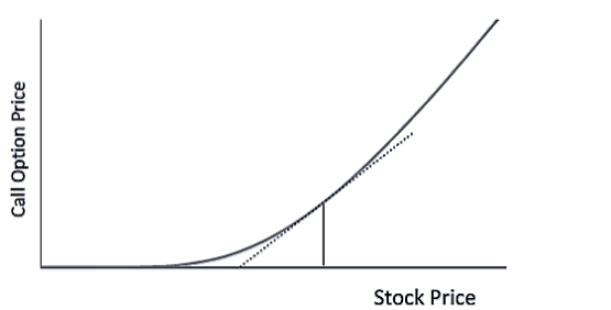
Let the price of a call option be c and the underlying stock price be S. Let ∆ be the sensitivity of the call option price to the stock price such that

$\Delta = \frac{\delta c}{\delta S}$

Where δS is a small change in the stock price, and δc is the corresponding change in the call option price.

The delta of a call option is the gradient illustrated by the dotted line in this figure.

A riskless position can be set up if one call option is sold and ∆ shares of the stock are bought. The cost of setting up the position is

S∆ – c

The position should earn the risk-free rate over the next short period of time.

This is similar to the argument used in valuation of options using binomial trees where the option position remained riskless for a single step of the tree. In this case, the period of time over which the option remains riskless is (in theory) infinitesimally short period of time.

The Pricing Formulas

Let $S_0$ is the current stock price, K is the strike price, T is the time to maturity in years, r is the risk-free rate per year (continuously compounded) for a maturity of T, and σ is an estimated volatility per year over the next T years. The Black-Scholes-Merton formulas for the price of a European call option (c) and a European put option (p) are

$c = S_0 N(d_1) - K e^{-rT} N(d_2)$

$p = Ke^{-rT} N(-d_2) - S_0 N(-d_1)$

where:

$d_1=\frac{\ln(S_0/K)+(r+\sigma^2/2)T}{\sigma\sqrt{T}}$

$d_2=\frac{\ln(S_0/K)+(r-\sigma^2/2)T}{\sigma\sqrt{T}}=d_1-\sigma\sqrt{T}$

The N function is the cumulative normal distribution function, and it can be calculated from NORMSDIST in Excel or from tables.

The Pricing Formulas – Example

Suppose the stock price is USD 56, the strike price is USD 60, the risk-free rate is 5% per annum, the volatility is 30% per annum, and the time to maturity is 18 months. In this case:
Put-Call parity states that when a European put option and a European call option on a non-dividend paying stock have the same strike price and time to maturity:

Call Price + PV of Strike Price = Put Price + Stock Price

Implied Volatility

Traders do use the Black-Scholes-Merton model, but not in exactly the way that Black, Scholes, and Merton originally intended. This is because they allow the volatility used to price an option to depend on its strike price and time to maturity.
In the BSM Model, volatility is an input and option price is the output.
To get implied volatility, option price is known and volatility is inferred.
Implied volatility isn’t based on historical pricing data on the stock. Instead, it’s what the marketplace is “implying” the volatility of the stock will be in the future, based on price changes in an option. Like historical volatility, this figure is expressed on an annualized basis.
•Market makers use implied volatility as an essential factor when determining what option prices should be. However, you can’t calculate implied volatility without knowing the prices of options. So some traders experience a bit of “chicken or the egg” confusion about which comes first: implied volatility or option price. In reality, it’s not that difficult to understand. Usually, at-the-money option contracts are the most heavily traded in each expiration month. If the options are liquid then the model does not usually determine the prices of the ATM options; instead, supply and demand become the driving forces. Then, once the at-the-money option prices are determined, implied volatility is the only missing variable. So it’s a matter of simple algebra to solve for it. After implied volatility is calculated for the at-the-money contracts in any given expiration month, pricing models and advanced volatility skews are used to determine implied volatility for other options that are less heavily traded.
In BSM model, volatility was assumed to be constant, but that is not the case. Volatility keeps on changing.
Implied volatility is typically of more interest to retail option traders than historical volatility because it’s forward-looking.
There is no analytic formula for implied volatility. Instead, it must be found using an iterative trial and error procedure.
One simple approach to determining implied volatility is called successive bisection.
Traders monitor implied volatilities carefully and often use them to communicate prices. If the assumptions underlying the Black-Scholes-Merton model hold exactly, then theoretically, for options with the same expiration date, the implied volatility is expected to be the same regardless of the strike price used. However, in reality, the implied volatility (IV) is different across the various strikes. This disparity is known as the volatility skew.
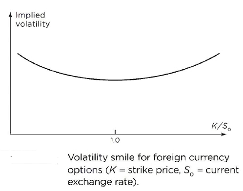
If the implied volatilities (IV) is plotted against the strike prices, a U-shaped curve might be obtained which resembles a smile. Hence, this particular volatility skew pattern is better known as the volatility smile.
The volatility smile used by traders to price foreign currency options has the general form shown in this figure. The implied volatility is relatively low for at-the money options. It becomes progressively higher as an option moves either into the money or out of the money.

Before the crash of 1987, there was no marked volatility smile for equity options. Since 1987, the volatility smile used by traders to price equity options (both on individual stocks and on stock indices) has had the general form shown in this figure. This is sometimes referred to as a volatility skew. The volatility decreases as the strike price increases. The volatility used to price a low-strike-price option (i.e., a deep-out-of-the-money put or a deep-in-the-money call) is significantly higher than that used to price a high-strike-price option (i.e., a deep-in-the-money put or a deep-out-of-the-money call).

More generally, traders monitor the volatility surface. This describes implied volatilities as a function of both strike price and time to maturity. When quoting options prices, traders interpolate between the known implied volatilities to determine an implied volatility for the option under consideration. This is then substituted into the Black-Scholes-Merton equation to determine the option price.

Options On Stock Indices (Dividends)

For a European option on a stock paying a continuous dividend yield at rate q, the formulae for the option prices become

$c = S_0 e^{-qT} N(d_1) - K e^{-rT} N(d_2)$

$p = Ke^{-rT} N(-d_2) - S_0 e^{-qT} N(-d_1)$

where

$d_1=\frac{\ln(S_0/K)+(r-q+\sigma^2/2)T}{\sigma\sqrt{T}}$

$d_2=\frac{\ln(S_0/K)+(r-q-\sigma^2/2)T}{\sigma\sqrt{T}}$

These formulas can be used for a European option on a stock index paying dividends at rate q when S_0 is the value of the index.

Options On Currencies

A foreign currency behaves like a stock paying a dividend yield at the foreign risk-free rate $(r_f)$ . The valuation equations are therefore obtained by setting $q=r_f$ to get

$c = S_0 e^{-r_f T} N(d_1) - K e^{-rT} N(d_2)$

$p = K e^{-rT} N(-d_2) - S_0 e^{-r_f T} N(-d_1)$

where $S_0$ is the current exchange rate, σ is its volatility, and:

$d_1 = \frac{\ln\left(\frac{S_0}{K}\right) + \left(r - r_f + \frac{\sigma^2}{2}\right)T}{\sigma \sqrt{T}}$

$d_2 = \frac{\ln\left(\frac{S_0}{K}\right) + \left(r - r_f - \frac{\sigma^2}{2}\right)T}{\sigma \sqrt{T}}$

Options On Futures

•A futures contract behaves like a stock paying a dividend yield at the domestic risk-free rate (r). The valuation equations are therefore obtained by setting q = r and $S_0=F_0$ to get

$c = F_0 e^{-rT} N(d_1) - K e^{-rT} N(d_2)$

$p = K e^{-r} N(-d_2) - F_0 e^{-rT} N(-d_1)$

where

$d_1 = \frac{ln\left(\frac{F_0}{K}\right) + \sigma^2\left(\frac{T}{2}\right)}{\sigma\sqrt{T}}$

$d_2 = \frac{ln\left(\frac{F_0}{K}\right) - \sigma^2\left(\frac{T}{2}\right)}{\sigma\sqrt{T}} = d_1 - \sigma\sqrt{T}$

The equations for pricing options on futures are referred to as Black’s model. The volatility parameter here (σ) is the volatility of the futures price.

As discussed in Financial Markets and Products, the forward price for a forward contract and the futures price for the corresponding futures contract can be approximately the same in many situations. Black’s model also gives the price of an option on a forward contract. Furthermore, a European put (call) option on the spot price of an asset is the same as a European put (call) option on the forward price of the asset when:
- They have the same strike price and time to maturity, and
- The forward contract matures at the same time as the option.

This result allows Black’s model to be used to value an option on the spot price of an asset in terms of the forward price of the asset. This is an approach often taken by traders because it avoids the need to estimate income on the asset (since the forward price captures all relevant aspects of the income).

Handling Discrete Dividends

The relevant dividends for valuing an option are those for which the ex-dividend date is during the life of the option. The relevant size of each dividend is the amount by which the stock price is expected to decrease on the ex-dividend date due to the dividend. The latter may be different from the amount of the dividend declared if capital gains are taxed differently from investment income.
If the present value of the dividends paid during the life of a European option is estimated as PV(D), the option can be valued by replacing S with S -PV(D) in the previous equations.

Example

Consider a six-month European put option on a stock whose price is USD 74. The strike price is USD 70, the risk-free interest rate is 5% per year (continuously compounded), and the volatility parameter is 20%. Additionally, dividends of USD 1.50 are expected with ex-dividend dates in one month and four months.

American Options

As discussed in Financial Markets and Products, call options on a non-dividend paying stock should never be exercised early. Hence the Black Scholes Merton model provides prices for American call options on non-dividend paying stocks as well as for European call options.
If dividends are sufficiently small so that some specific mathematical conditions are satisfied, an American call option on a dividend-paying stock can be valued as a European call option.
American put options on stocks and American call and put options on stock indices, currencies, and futures should not be valued as European options. Binomial trees can be used for valuation in these cases.

Warrants

Warrants are options issued by a company on its own stock. If warrants are exercised, the company issues more shares, and the warrant holder buys the shares from the company at the strike price. An option traded by an exchange does not change the number of shares issued by a company. However, a warrant allows new shares to be purchased at a price lower than the current market price. This dilutes the value of existing shares.
Assuming markets are efficient, the share price will reflect the potential dilution from outstanding warrants. This means that warrants can be valued in the same way as exchange-traded options once they have been announced.
A firm that is deciding whether or not to issue warrants might be interested in calculating the cost of the warrants to its existing shareholders. If there are N existing shares, and the company is contemplating the issue of M warrants (with each giving the warrant holder the right to buy one new share), it can be shown that the cost of each warrant to existing shareholders is N/(N + M) multiplied by the price of each warrant. The price of each warrant is calculated in the same way as the price of an exchange-traded option and is based on the share price before the warrant issue was announced.

Contact us

The Black-Scholes-Merton Model

Learning Objectives

Chapter Contents

Introduction

Stock Price Movements

Return Calculations

Volatility

Measuring Time

Assumptions

No-Arbitrage For Options

The Pricing Formulas

The Pricing Formulas – Example

Implied Volatility

Options On Stock Indices (Dividends)

Options On Currencies

Options On Futures

Handling Discrete Dividends

American Options

Warrants

Previous Chapter

Next Chapter

Go to Syllabus

Courses Offered

By : Micky Midha

VIEW DETAILS

By : Micky Midha

VIEW DETAILS

By : Micky Midha

VIEW DETAILS

By : Micky Midha

VIEW DETAILS

By : Shubham Swaraj

VIEW DETAILS

FAQs

No comments on this post so far:

Add your Thoughts:

Quick Links

Company