Introduction

• The analysis and use of interest rates is central to finance. There are different types of interest rates along with different modes of measurement.
• The interest rate term structure describes how interest rates vary depending on their maturity. In an upward-sloping term structure, long-term interest rates are higher than short-term interest rates. In a downward-sloping term structure, the opposite is true.
• An interest rate is the return earned by a lender when advancing funds to a borrower.
  • A major factor in determining an interest rate is the risk that the borrower will default and not repay the lender in full; this risk is called credit risk. As the credit risk increases, the interest rate required by the lender from the borrower also increases.
  • Another factor in determining interest rates is liquidity; in this context, liquidity refers to the ease with which an interest-bearing instrument can be sold from one investor to another at a competitive price.
• Interest rates (and the spreads between different interest rates) are often expressed in basis points. One basis point is 0.01%.

Categories Of Rates

Government Borrowing Rates

• One important interest rate is that paid by a government on its borrowings in its own currency. In the United States, this is referred to as the Treasury rate. It is considered highly unlikely that the government of a developed country will default on debt issued in its own currency. This is because a government can always create more currency to meet its obligations. As a result, government debt from developed countries is considered to be risk-free and the interest rates on these borrowings are generally below those on other borrowings in the same currency.

Libor

• The London Interbank Offered Rate (Libor) has historically been an important reference rate in financial markets. Libor interest rates are compiled from the estimated unsecured borrowing costs of 18 highly rated global banks. These estimates are made daily (just prior to 11 a.m. in London) for five different currencies and seven borrowing periods ranging from one day to one year. The highest and lowest four quotes for each estimate are discarded and the remainder are averaged to determine the daily Libor fixings.
• Banks have been accused of trying to manipulate Libor rates by providing overly high or low estimates of their borrowing rates. A bank might have an incentive to do this when the payoff from a derivative it has entered depends on a specific Libor fixing for that day. Another scenario would be a bank that reports excessively lower rates in order to appear more creditworthy.
• The underlying problem is that there is not enough Libor borrowing for estimates to be based on actual transactions. As a result, the person providing the estimates has to use quite a bit of judgment. There are plans to begin phasing out Libor in 2021 and replace it with a rate based on actual transactions (rather than estimates). Two main candidates for this replacement benchmark rate are: the repo overnight rate and the overnight interbank borrowing rate.
• The United States has proposed the use of the repo-based Secured Overnight Financing Rate (SOFR). Meanwhile, the United Kingdom has proposed the use of the Sterling Overnight Index Average (SONIA), which is based on interbank borrowing. Both are one-day rates. Swaps are necessary to create a complete interest rate term structure from these rates.

Repo Rate

• In a repo agreement, securities are sold by Party A to Party B for a certain price with the intention of being repurchased at a later time at a higher price. Suppose that the initial price paid by B to A for the securities is X and the price at which they will be repurchased is X+e. The effect of the repo is that Party B has lent X to Party A for an amount of interest equal to e.
• If Party A fails to repurchase the securities as agreed, Party B can simply keep the securities. This means that Party B takes very little risk, provided that:
  • The value of the securities equals (or is very close to) X, and
  • This value is fairly stable.
• Party B is in a better position than it would be if the securities had been merely pledged as collateral. This is because the repo leads to Party B owning the securities without having to initiate legal action to gain possession. Repos lasting one day (i.e., overnight repos) are the most common, but longer-term repos exist as well.

Overnight Interbank Borrowing

• In many countries, banks are required to keep cash in reserve with the central bank, which depends on each bank's outstanding liabilities. At the end of each day, some banks have excess reserves, while others have a shortage. This leads to the practice of overnight interbank lending.
• In the US, the interest rate on this overnight lending is referred to as the federal funds rate. The weighted average of the rates in these transactions is termed the effective federal funds rate. The Federal Reserve monitors this rate and periodically intervenes with its own trades to increase or decrease the rate. The respective average overnight rates in the UK and the Eurozone are the Sterling Overnight Index Average (SONIA) and the Euro Overnight Index Average (EONIA).

Swaps

• For this chapter, swaps are a way in which long-term rates are created from short-term rates to create a complete interest rate term structure. Swaps can be used to create an interest rate term structure from observed one-day rates. A three-month overnight indexed swap is an agreement to exchange the geometric average of the daily effective federal funds rates over the following three months for a pre-determined fixed rate (with both rates being applied to the same principal). Meanwhile, a five-year swap is one in which it is agreed that the exchange just described will take place every three months for the next five years.

Risk-Free Rates

• The risk-free rates used to value derivatives are determined from overnight interbank rates using overnight indexed swaps. Treasury rates are not used because they are considered to be artificially low. Two reasons for this are as follows.

1. Banks are not required to keep capital to support an investment in Treasury instruments, but they are required to keep capital for other very low-risk instruments.
2. In some countries (e.g., the United States), the income from Treasury instruments is given favorable tax treatment.

Compounding Frequency

• In order to fully understand a quoted interest rate, it is necessary to know the compounding frequency with which it is measured. The compounding frequency defines the extent to which interest is earned on interest.
• This table denotes the value to which USD 100 grows at 5% as the compounding frequency is varied.

Compounding Frequency	Value of USD 100 at the End of Five Years (USD)
Annual	121.55
Semi-Annual	121.84
Quarterly	121.99
Monthly	122.09
Weekly	122.13
Daily	122.14

• Just as pounds and grams are alternative units of measurement for weight, annual compounding and semi-annual compounding can be considered as alternative units of measurement for interest rates.
• The general formula for the future value of an amount A when it is invested at rate R for T years when R is expressed with a compounding frequency of m times per year is

• Suppose R₁ is an interest rate when compounding is m₁ times per year and R₂ is the equivalent rate when compounding is m₂ times per year. The future values are the same if:

This means that:

This can be rewritten as:

• Suppose an interest rate is 8% per year with annual compounding. Find the equivalent rate which should be expressed with quarterly compounding.
• Suppose an interest rate is 10% per year with monthly compounding. Find the equivalent rate which should be expressed with semi-annual compounding.

Compounding Frequency – Usual Conventions

• The usual convention is that interest rates are expressed so that the compounding frequency corresponds to the frequency with which payments are made.
• Instruments that last one year or less (from date of issue) are termed money market instruments; their principal and interest are both paid at maturity. An interest rate on a three-month money market instrument is therefore typically quoted with quarterly compounding, the interest rate on a one-year money market instrument is typically quoted with annual compounding, and so on. This convention can be misleading. If the one-year money market interest rate is 10% and the one-month money market interest rate is 9.8%, it may appear as though the one-year rate is greater than the one-month rate. However, the 9.8% is measured with monthly compounding, while the 10% is measured with annual compounding.
• In the United States and some other countries, bonds which last longer than one year (from date of issue) normally pay interest every six months. The yield provided by a bond is therefore normally expressed with semi-annual compounding.

Compounding Frequency – Usual Conventions Exceptions

• Sometimes the compounding frequency does not reflect the frequency of payments. In Canada, for example, mortgage interest rates are expressed with semi-annual compounding even though payments are made every month (or every two weeks). In the United States, this mortgage interest rate would be expressed with monthly compounding; in the United Kingdom, it would be expressed with annual compounding. These varied ways of expressing interest rates are regulatory requirements designed to allow borrowers to compare interest rates with as little confusion as possible.

Continuous Compounding

• Continuous compounding is used in the valuation of options and other, more complex derivatives. It can also be convenient to work with continuously compounded interest rates and yields when considering futures prices. The formulas involving interest rates expressed with continuous compounding are actually simpler than those involving periodic compounding.
• Suppose R_m is an interest rate expressed with compounding m times per year and R_c is the same rate expressed with continuous compounding. The future values are the same if:

So that

and

• Suppose an interest rate is 6% per year with semi-annual compounding. Find the equivalent rate which should be expressed with continuous compounding.
• Suppose an interest rate is 9% per year with continuous compounding. Find the equivalent rate which should be expressed with quarterly compounding.

Zero Rates

• A zero-coupon interest rate (or zero rate or spot rate) for maturity T is the applicable interest rate when an investor receives the total return (interest and principal) at the end of T years.
• Instruments with maturities of one year or less usually provide all principal and interest at the ends of their lives. They therefore provide zero rates directly. Most instruments that (when issued) last longer than one year provide regular interest payments known as coupons. Zero rates must then be determined using bootstrapping method.
• The present value of an amount A received at time T when the interest rate R is expressed with a compounding frequency of m times per year is

• The discount factor is the amount by which the cash flow is multiplied to get the present value.
• When the interest rate R is compounded continuously, then

Bond Valuation

• The valuation of a bond involves identifying its cash flows and discounting them at the interest rates corresponding to their maturities. As an example, suppose that zero-coupon interest rates with semi-annual compounding are those shown in this table

Maturity (Years)	Zero-Coupon Interest Rate (Semi-Annually Compounded)
0.5	3.0%
1.0	3.8%
1.5	4.4%
2.0	4.8%
2.5	5.1%
3.0	5.3%

Consider a three-year bond with a principal of USD 100. The principal is also known as the par value (also known as the face value) and it is the amount that must be repaid at maturity. In this example, the maturity is three years.

Suppose further that the bond provides semi-annual coupons at the rate of 6% per year every six months. This means that the bond provides interest of USD 3 every six months. To value the bond, the cash flows are discounted at the interest rates corresponding to the times when they are received and then sum the results.

• This table presents the cash flows from the bond in this example

Time (Years)	Cash Flow (USD)
0.5	3
1.0	3
1.5	3
2.0	3
2.5	3
3.0	3

• The present value of the first cash flow (received at time 0.5 years) is

Similarly, the present value of the other cash flows are –

• These results are summarized in this table

Time (Years)	Cash Flow (USD)	Discount Factor	Present Value (USD)
0.5	3	0.9852	2.9557
1.0	3	0.9631	2.8892
1.5	3	0.9368	2.8104
2.0	3	0.9095	2.7285
2.5	3	0.8817	2.6541
3.0	103	0.8548	88.0407
Total			102.0695

The value of the bond itself can be shown to be USD 102.0695. This is greater than USD 100 because the coupon rate earned on the bond is 6% per year (which is higher than the rates at which the bond's cash flows are being discounted).

Bond Valuation – Bond Yield

• The return earned by an investor on a bond is often described by what is termed the bond yield. This is the discount rate that equates the present value of all the cash flows to the market price.
• For the bond in the previous example, the bond yield y (semi-annually compounded) is the solution to the equation

The solution can be found using an iterative trial-and-error procedure. (Solver in Excel is a useful resource.) The solution for the above is y=5.2455%.

Hence, the bond provides a yield of 5.2455% (with semi-annual compounding).

Bond Valuation – Par Yield

• The par yield of a bond is the coupon rate that would cause the value of the bond to equal its par value.
• For example, consider the rates in the previous interest rate table with a par value of USD 100. If the par rate (paid semi-annually) on a three-year bond is c, the par yield would satisfy

= 100

Bond Valuation

• Defining terms:
  • m: The frequency with which coupons are paid (i.e. the frequency of compounding)
  • A: The value of an annuity that pays USD 1 on each coupon payment date, and
  • d: The present value of USD 1 received at bond maturity (i.e. the discount factor)

• The value of coupons is
  . The value of the final principal is 100d. If c is the par yield, we therefore require

This can be rewritten to have c equal to:

In the previous example, m = 2, A = 5.5310, and d = 0.8548

Time Value Of Money Recap

• Whenever TVM calculations are made, the period of time associated with the frequency of cash flows must match the compounding frequency for the discounting or compounding rate. To address any differences,
  • Make any necessary adjustment to convert the stated annual rate to the appropriate periodic rate as

• Make any necessary adjustment to the time index to account for the compounding frequency as

Duration

• Yield duration measures the sensitivity of a bond's price to a change in its yield. The approximate duration relationship is

This is equivalent to:

where

B is the price of a bond,

D is the bond's duration,

is the change in the bond's yield, and

 is the change in the bond's price resulting from the change in the yield.

• The value of the duration (D) depends (slightly) on the compounding frequency with which the yield (y) is measured. The Macaulay duration is the correct value of D if the yield is measured with continuous compounding. The modified duration is the correct duration to use when D is measured with some other compounding frequency.

Duration Example 1

Duration Example 2

• Consider the bond in the topic – Properties of Interest Rates (Part 1).

Time (Years)	Cash Flow (USD)	Discount Factor	Present Value (USD)
0.5	3	0.9852	2.9557
1.0	3	0.9631	2.8892
1.5	3	0.9368	2.8104
2.0	3	0.9095	2.7285
2.5	3	0.8817	2.6541
3.0	103	0.8548	88.0407
Total			102.0695

The price of the bond is USD 102.0695 and the yield was calculated as 5.2455% with semi-annual compounding. With continuous compounding, the yield is obtained as

or 5.1779%.

• The Macaulay duration calculation is illustrated in this table.

Time (Years)	Cash Flow	Present Value Using Yield as Discount Rate	Weight	Time × Weight
0.5	3	2.9233	0.02864	0.01432
1.0	3	2.8486	0.02791	0.02791
1.5	3	2.7758	0.02720	0.04079
2.0	3	2.7049	0.02650	0.05300
2.5	3	2.6357	0.02582	0.06456
3.0	103	88.1811	0.86393	2.59180
Total		102.0695	1.00000	2.79238

When discounted at the yield, the first cash flow has a present value of USD 2.9233. This is 2.864% of the total present value. The amount of weight given to T=0.5 in the calculation of Macaulay duration is therefore .

Modified Duration

• When rates are compounded m times per year, instead of continuous compounding, then modified duration is used

Dollar Duration

• Dollar duration is another measure that is sometimes used. This is the product of the modified duration and the price of the bond. If dollar duration is , then

• Whereas D provides the sensitivity of proportional changes in a bond's price to a change in its yield, provides the sensitivity of actual changes in a bond's price to changes in its yield.

Limitations of Duration

• A major issue with duration is that it assumes a linear relationship between interest rates and bond price. But actually, the relationship is non-linear and the graph of bond price versus yield is curved. The extent of the deviation from a linear relationship or the degree to which the graph is curved is known as convexity. The higher the convexity, the more inaccurate duration is for measuring interest rate sensitivity.
• Duration provides a good approximation of the effect of
  • a small
  • parallel shift

in the interest rate term structure.

When all interest rates change by a certain amount, the yield on a bond changes by almost the same amount.

However, if the change in the bond yield arises from

• a non-parallel shift in the interest rate term structure, or
• the change being considered is large.

then bond price change based on duration alone does not provide a good approximation for the price change.

Convexity

• The impact of parallel shifts in the interest rate term structure can be measured more accurately by considering convexity in addition to duration. If C is convexity, then

This equation allows relatively large parallel shifts to be considered.

• The calculation of convexity is similar to the calculation of duration, except that the weight is multiplied by the square of time (rather than just the time).
• When rates are expressed with compounding m times per year, then modified convexity is defined as

• Table 16.6 Calculation of convexity for the same bond considered earlier

Time (Years)	Square of Time	Cash flow	PV Using as Discount Rate	Weight	Square of Time × Weight
0.5	0.25	3	2.9233	0.02864	0.00716
1.0	1. 00	3	2.8486	0.02791	0.02791
1.5	2.25	3	2.7758	0.02720	0.06119
2.0	4.00	3	2.7049	0.02650	0.10600
2.5	6.25	3	2.6357	0.02582	0.16139
3.0	9.00	103	88.1811	0.86393	7.77539
Total			102.0695	1.00000	8.13904

Forward Rates

• Forward rates are the future interest rates implied by today's zero-coupon interest rates.

• Consider again the rates in the following table which was also provided in FMP 16 (Part 1).

• The corresponding forward rates have been calculated and presented in the following table. Your task is to verify all the results and let us know in the forum if you need any help.

Maturity (Years)	Zero-coupon Interest Rate (semi-Annually Compounded)
0.5	3.0%
1.0	3.8%
1.5	4.4%
2.0	4.8%
2.5	5.1%
3.0	5.3%

Period	Forward Rate
0.5 year to 1.0 year	4.603%
1.0 year to 1.5 years	5.605%
1.5 years to 2.0 years	6.005%
2.0 years to 2.5 years	6.304%
2.5 years to 3.0 years	6.303%

Forward Rate Agreement

• A forward rate agreement (FRA) can be thought of as an agreement to apply a certain interest rate to a certain principal for a certain period in the future. Formally, it is an agreement that a pre-specified fixed interest rate will be exchanged for a floating interest rate (with both being applied to a certain principal for a certain period). The floating interest rate is usually Libor.
• Example –

Suppose an FRA involves paying a fixed interest rate of 4% and receiving the three-month Libor on a principal of USD 1 million for the three-month period beginning in one year. If the three-month Libor fixing in one year proves to be 4.8%, the FRA will involve interest being paid at a rate of 4% and received at a rate of 4.8%. Because these are money market rates, they are expressed with a compounding frequency corresponding to their maturity. (In this case, they are expressed with quarterly compounding.)

Forward Rate Agreement Example

Consider the same example given in the previous two slides.

Forward Rate Agreement

• An interest rate swap, which will be discussed in a later chapter can be regarded as a portfolio of FRAs. Each exchange in an interest rate swap is an agreement to exchange a pre-specified fixed interest rate for a floating interest rate (again, with both applied to a certain principal).

• Interest is normally paid at the end of the period to which it applies. By convention, however, an FRA is usually settled at the beginning of the period covered by the FRA. The settlement amount is therefore the present value of the difference in interest amounts (with the discount rate being the floating Libor rate). Expressed algebraically, the payoff is

where

R is the realized floating rate,

is the fixed rate,

L is the principal to which the rates are applied, and

 is the length of the time period.

For the party on the other side of the transaction (who pays floating and receives fixed), the payoff is

• An FRA can be valued by assuming that the forward Libor will occur. Expressed algebraically, the value of an FRA where floating is received and fixed is paid is

where

is the forward rate for the period underlying the FRA and

PV denotes the present value (using the risk-free rate) from the beginning of the period covered by the FRA to today.

Similarly, the value of an FRA where floating is paid and fixed is received is

Determining Zero Rates

• Money market instruments lasting less than one year provide their entire return at the end of their lives. Thus, they provide information about their zero-coupon interest rates in a direct way. However, instruments lasting longer than one year usually make regular payments prior to maturity. It is then necessary to calculate the zero-coupon rates implied by these instruments. One way of doing this is by working forward and fitting the zero-coupon rates to progressively longer maturity instruments. This is called the bootstrap method.
• Example –

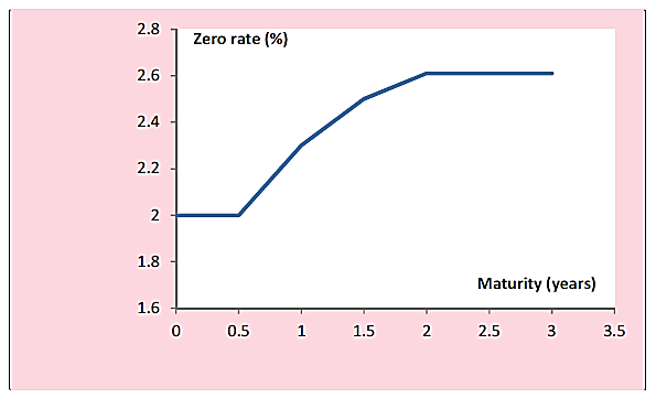
Suppose the zero-coupon interest rates (semi-annually compounded) for maturities of 0.5, 1.0, and 1.5 years have already been determined. and are given in this table.

Maturity (Years)	Zero-Coupon Interest Rate Semi-Annually Compounded
0.5	2.0%
1.0	2.3%
1.5	2.5%

• Suppose further that a two-year bond with a par value of USD 100 has a market value of USD 102.7 when it pays a (semi-annual) coupon at the rate of 4% per year. If the two-year zero-coupon interest rate is R, the equation that equates the value of the bond to USD 102.7 is

• A zero curve defines the relationship between zero-coupon interest rates and their maturities. The zero-coupon interest rates in a zero curve are usually assumed to be constant until the first maturity for which data is available. They are also usually assumed to be constant beyond the longest maturity for which data is available. The zero curve for previous example will be as in this figure.

• The calculations to produce a piecewise linear zero-rate curve are not always as straightforward as in the case above. For example, suppose the next price available was for a 2.4-year bond (instead of a two-year bond). The 2.4-year zero rate equal to R. Because a coupon is paid on the bond at the 1.9-year point, the zero rate for a maturity of 1.9 years has to be determined in terms of R. By interpolating between the 1.5-year rate of 0.025 and the 2.4-year rate of R, the 1.9-year rate has to be estimated

Theories of the Term Structure

• There are several theories about what determines the shape of the zero-coupon interest rate term structure.
• One is known as the market segmentation theory. This argues that short- , medium- , and long-maturity instruments attract different types of traders. While short-maturity rates would be determined by the activities of traders who are only interested in short-maturity investments, medium- and long-maturity instruments would only attract traders interested in those investments.

It is now generally recognized that the market segmentation theory is unrealistic. Market participants do not focus on just one segment of the interest rate term structure. For example, pension plans are primarily interested in trading long-maturity bonds, but will move to medium- or short-maturity instruments if their yields seem more attractive.

Another theory is known as the expectations theory. This argues that the interest rate term structure reflects where the market is expecting interest rates to be in the future. If the market expects interest rates to rise, the term structure of interest rates will be upward-sloping (with long-maturity rates being higher than short-maturity interest rates). If the market expects interest rates to decline, then the term structure will be downward-sloping (with long-maturity rates being lower than short-maturity rates). Expectations theory argues that forward rates should be equal to expected future spot rates.

In practice, interest rate term structures are upward-sloping much more often than they are downward-sloping. This raises questions over the expectations theory, because it can reasonably hypothesized that the market expects interest rates to decrease as often as it expects interest rates to increase. If the expectations theory were correct, we would expect to see downward-sloping term structures occurring as often as upward-sloping term structures.

• A third theory, known as the liquidity preference theory, is capable of explaining this disparity. The theory argues that if the interest rate term structure reflects what the market expects interest rates to be in the future (i.e., the expectations theory holds), most investors will choose a short-term investment over a long-term investment. This is because of liquidity considerations. A short-maturity investment means that the funds will be available earlier to meet any needs (anticipated or unforeseen) that arise.

The choice between long-maturity and short-maturity instruments can be also perceived from the perspective of the borrower. Short maturity borrowing usually has to be rolled over into new borrowing at the end of its life. This also entails liquidity risks. If (rightly or wrongly) the market's view of the financial

health of the borrower declines, it may not be possible for the company to roll over short-term borrowing at a competitive interest rate.

Liquidity considerations therefore lead to lenders wanting to lend for short periods of time and borrowers wanting to borrow for long periods of time. In order to match borrowers and lenders, financial intermediaries (such as banks) must increase long-term rates relative to the market's expectations about future short-term rates. As they do this:

• Long-term borrowing becomes less attractive because short-term rates are more attractive to borrowers, and
• Short-term lending becomes less attractive because long-term rates are more attractive to lenders.

Liquidity preference theory therefore argues that the process of matching borrowers and lenders leads to long rates being higher than the market's expectations would suggest. To be precise, it argues that forward rates consistently overstate expected future spot rates.

Theories of the Term Structure Example

• Suppose that only two rates are offered in the market: a three-month rate and a five-year rate. Suppose further that both rates are 2.5% per year and that this reflects the market's expectations (so that all expected future three-month rates are 2.5% per year). If the term structure of interest rates is flat at 2.5% (consistent with expectations theory), liquidity considerations will lead lenders to choose to commit funds for only three months, while borrowers will choose the five-year maturity. This will lead to a mismatch. As financial intermediaries try to match borrowers and lenders, market forces will lead to the five-year rates being pushed above 2.5%. For example, it might be found that making the five-year rate 3.5% (while keeping the three-month rate at 2.5%) will cause some borrowers to switch from five-month borrowing to three-month borrowing and some lenders to switch in the other direction. The end result is that supply and demand are matched at both maturities.