Introduction

• Probability can be used to describe any situation with an element of uncertainty. However, random variables restrict attention to uncertain phenomena that can be described with numeric values.
• Two functions are commonly used to describe the chance of observing various values from a random variable: the probability mass function (PMF) and the cumulative distribution function (CDF).
• Moments are used to summarize the key features of random variables. A moment is the expected value of a carefully chosen function designed to measure a characteristic of a random variable.
• The quantile function is the inverse of the CDF. It defines two moment-like measures: the median (which measures the central tendency of a random variable) and the interquartile range (which is an alternative measure of spread).
• Continuous random variables produce values that lie in a continuous range.

Definition Of A Random Variable

• Random variables limit attention to random phenomena, which can be described using numeric values.
• A random variable is a function of 𝜔 (i.e., an event in the sample space Ω) that returns a number x.

  

• Univariate random variables are frequently distinguished based on the range of values produced.
• A discrete random variable is one that produces distinct values.
• A continuous random variable produces values from an uncountable set, (e.g., any number on the real line ℝ).
• The key properties of discrete and continuous random variables are identical.

Discrete Random Variables

• A discrete random variable assigns a probability to a set of distinct values. This set can be either finite or contain a countably infinite set of values.
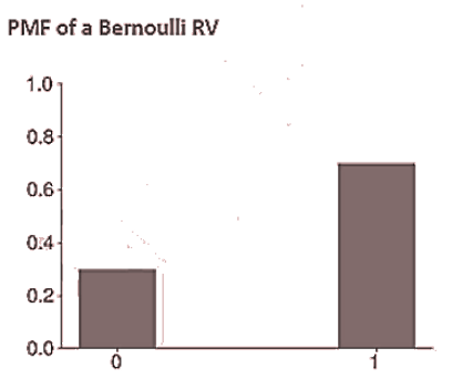
• The set of values that the random variable may take is called the support of the function. For example, the support for a Bernoulli random variable is {0,1}.
• Two functions are frequently used when describing the properties of a discrete random variable’s distribution –
  • PMF
  • CDF
• The PMF returns the probability that a random variable takes a certain value. Any PMF must have two properties.
  1. The value returned from a PMF must be non-negative.
  2. The sum across all values in the support of a random variable must be one.
• In the case of a Bernoulli random variable, the PMF is given by

  

  

• The cumulative distribution function CDF measures the total probability of observing a value less than or equal to the input 𝑥 (i.e., ).
• In the case of a Bernoulli random variable, the CDF is a simple step function:

  

  

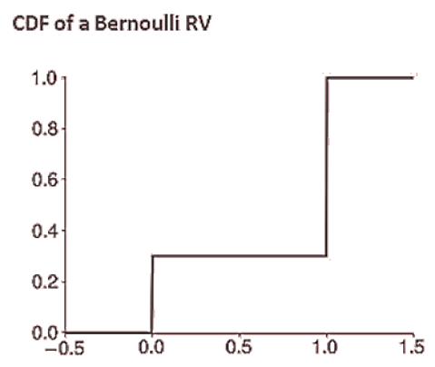
• The CDF can always be expressed as the sum of the PMF for all values in the support that are less than or equal to 𝑥:

  

  where R(X) is used to denote the range of realizations that may be produced from the random variable 𝑋 and ϵ means “an element of.”

• Conversely, the PMF is the difference of the CDFs evaluated at consecutive values in the support of X. For a Bernoulli random variable:

  

  for  .

Expectations

• The expected value of a random variable X is the weighted average of all possible outcomes for that variable, where the weights are the probabilities of the occurrence of those outcomes i.e.

  

  For Example, the expected value in a roll of a fair die is given by

  

  Although 3.5 can never be obtained in a single roll of a die, but the average of all outcomes in the long run will approach 3.5, and the expected value denotes that only.

  Another example

  When X is a Bernoulli random variable where the probability of observing 1 is p:

  E[X]=0×(1-p)+1×p=p

• Functions of random variables are also random variables and therefore have expected values. The expectation of a function 𝑓 of a random variable X is defined as:

  

  where f(x) is a function of the realization value x

  For example, when X is a Bernoulli random variable, then the expected value of the exponential of X is

  

Expectations – Example

A stock X is priced at $12. There is a 20% probability that the stock will go up to $16, a 50% probability that the stock will remain $12, and a 30% probability that the stock will go down to $7 after one year. Find the expected stock price after one year. If the required rate of return is 8%, find whether it is undervalued or overvalued today.

Expectations – Properties

• The expectation operator has one particularly useful property in that it is a linear operator.
• An immediate implication of linearity is that the expectation of a constant is the constant i.e.

  E[a]=a

• A related implication is that the expectation of the expectation is just the expectation, i.e.

  E[E[X]]=E[X]

• Furthermore, the expected value of a random variable is a constant (and not a random variable).
• The expectation operator does not pass through nonlinear functions of X. For nonlinear functions, in general:

  For example,

  

  Some properties can be mathematically summarized as follows :

  • E(cX)=cE(X), where c is a constant.
  • E(X+Y)=E(X)+E(Y), where X and Y are any random variable.
  • E(cX+a)=cE(X)+a, where c and a are constants.
  • E(XY)=E(X)E(Y), where X and Y are independent random variables.
  • E(XY)≠E(X)E(Y), if X and Y are not independent.
  • , where X is a random variable.

Expectations – Properties – Example

• Find expected value of Y if the relationship between X and Y is given by:

• The following data is given regarding expected values of X and its higher powers:

, ,

Expectations – Jensen’s Inequality

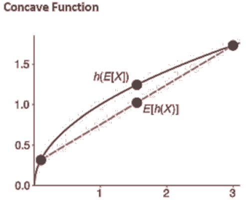
• Jensen’s inequality is a useful rule that provides some insight into the expectation of a nonlinear function of a random variable. Jensen’s inequality applies when a nonlinear function is either concave or convex.
  • A function g(x) is concave if for all 𝑡 in the interval [0,1] and x in the domain of g.
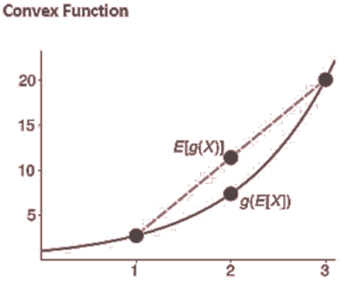
  • A function h(𝑥) is convex if for all t in the interval [0,1] and x in the domain of h.
• If h(X) is a concave function of X, then E[h(x)]< h(E[X]).

  

• If g(X) is a convex function of X, then E[g(X)]>g(E[X]).

  

Expectations – Jensen’s Inequality – Example

As an example of a convex function, suppose you play a game in which you roll a die and receive the square of the number rolled. Let X represent the die roll. We have that the payoff function is . Then:





And

Moments

• Moments are a set of commonly used descriptive measures that characterize important features of random variables. Specifically, a moment is the expected value of a function of a random variable.
• The first moment is defined as the expected value of 𝑋:

  

• The second and higher central moments are defined as:

  

  where r denotes the order of the moment (2 for the second, 3 for the third, and so on).

• Non-central moments are not centered around the mean and are defined as:

  

• Non-central moments and central moments contain the same information and the central moment can be directly constructed from the first 𝑟 non-central moments. For example, the second central moment can be calculated as:

  Note that the first central and non-central moments are the same:

  

• There are four common moments: the mean, the variance, the skewness, and the kurtosis. The mean is the first moment and is denoted

  μ=E[X]

  The mean is the average value of 𝑋 and is also referred to as the location of the distribution.

• The variance is the second moment. The variance of a random variable measures its unpredictability or noise by determining the degree to which the values of a random variable differ from its expected value. It is denoted by σ^2 and defined as the expected value of the square of the difference between the variable and its mean i.e.

  

• The square root of variance, (i.e. ), denoted by σ, is known as the standard deviation, and is a measure of volatility of a random variable. A low standard deviation indicates that the values are close to the mean (or expected value) of the set, while a high standard deviation indicates that the values are more spread out over a wider range. It is a commonly reported alternative to the variance, as it is a more natural measure of dispersion and is directly comparable to the mean (because the units of measurement of the standard deviation are the same as those of the mean).
• The third moment is skewness which is defined as:

  

  The skewness measures asymmetry in a distribution, because the third power depends on the sign of the difference. Negative values of the skewness indicate that the chance of observing a large (in magnitude) negative value is higher than the chance of observing a similarly large positive value. Asset returns are frequently found to have negative skewness.

• The fourth standardized moment, known as the kurtosis, is defined as:

  

  Specifically, the kurtosis of a random variable is commonly benchmarked against that of a normally distributed random variable, which is 3. Random variables with kurtosis greater than 3 are described as being heavy-tailed/fat-tailed (i.e., having excess kurtosis). Financial return distributions have been widely documented to be heavy-tailed.

Moments – Standardizing Random Variables

• When X has mean μ and variance σ^2, a standardized version of X can be constructed as

  

  This variable has mean 0 and unit variance (and standard deviation).

Moments – Moments And Linear Transformations

• Many variables used in finance and risk management do not have a natural scale. For example, asset returns are commonly expressed as proportions or (if multiplied by 100) as percentages. This difference is an example of a linear transformation.
• Let Y=a+bX , where 𝑎 and b are both constant values. It is common to refer to a as a location shift and b as a scale, because these directly affect the mean and standard deviation of Y.

  The mean of Y is E[Y]=a+bE[X]

  The variance of 𝑌 is or equivalently

• The location shift a has no effect on the variance because the variance measures deviations around the mean. The standard deviation of Y is

  

  The standard deviation is also insensitive to the shift by a and is linear in b.

• If b >0, then the skewness and kurtosis of 𝑌 are identical to the skewness and kurtosis of X.
• If 𝑏 <0, then the skewness has the same magnitude but the opposite sign. This is because it uses an odd power (i.e., 3). The kurtosis, which uses an even power (i.e., 4), is unaffected when b<0.

Continuous Random Variables

• A continuous random variable is one with a continuous support.
• Continuous random variables use a probability density function (PDF) in place of the probability mass function. The PDF f(X) returns a non-negative value for any input in the support of X. Note that a single value of f(X) is technically not a probability because the probability of any single value is always 0. This is necessary because there are infinitely many values 𝑥 in the support of X.
• A PMF is required to sum to 1 across the support of X. This property also applies to a PDF, except that the sum is replaced by an integral:

  

• The CDF of a continuous random variable is identical to that of a discrete random variable. It is a function that returns the total probability that the random variable X is less than or equal to the input (i.e., ).
• The PDF can be derived from the CDF by taking the derivative:

  

  Conversely, the CDF is the integral of the PDF up to 𝑥:

  

• The expectation of a continuous random variable is also an integral. The mean E[X] is
  

Quantiles And Modes

• For a continuous or discrete random variable 𝑋, the is the smallest number q such that . This is traditionally denoted by:
  
  where

  and

  inf⁡ selects the smallest possible value satisfying the requirement that .

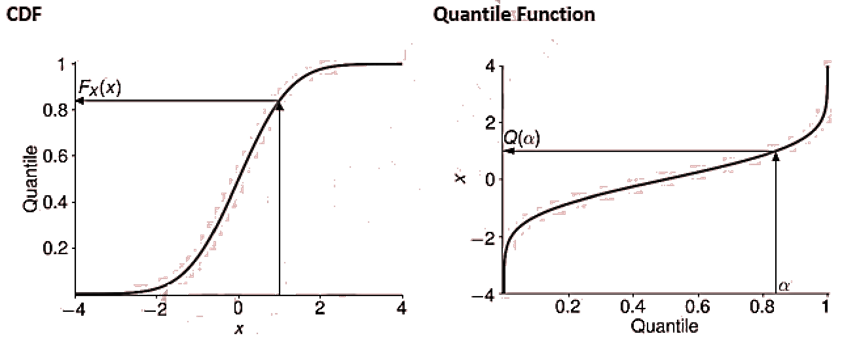
• The quantile function can be defined as such that returns the q of X and:

  

  so that the quantile function is the inverse of the CDF. Recall that the CDF transforms values in the support of X to the cumulative probability. These values are always between 0 and 1. The quantile function thus maps a cumulative probability to the corresponding quantile.

  

• The median is defined as the 50% quantile and measures the point that evenly splits the probability in the distribution (i.e., so that half of the probability is below the median and half is above it).
• The median is the middle reading in a data set when all the data are ranked in ascending order.
• To find the median value in a list with an odd amount of numbers, we find the number that is in the middle with an equal amount of numbers on either side of the median. For example, consider:

  7%, 11%, 9%, 4%, -3%,-5%,-2%,6%,11%

• In case when the number of observations are even, the median is the average of the two numbers in the middle. For example, consider all 10 returns of our last example:

  7%, 11%, 9%, 4%, -3%,-5%,-2%,6%,11%,15%

• The interquartile range (IQR) is defined as the difference between the 75% and 25% quantiles. It is a measure of dispersion that is comparable to the standard deviation. The IQR is less sensitive to changes in the extreme tail of a distribution.
• Quantiles are also noteworthy because they are always well-defined for any random variable. Moments, even the mean, may not be finite when a random variable is very heavy-tailed. The median, or any other quantile, is always well-defined even in cases where the mean is not.
• The mode is a measure of common tendency. It measures the location of the most frequently observed values from a random variable. When a random variable is continuous, the mode is the highest point in the PDF.