Introduction

• There are three common discrete distributions:
  • The Bernoulli is a general purpose distribution that is typically used to model binary events.
  • The binomial distribution describes the sum of 𝑛 independent Bernoulli random variables.
  • The Poisson distribution is commonly used to model hazard rates, which count the number of events that occur in a fixed unit of time (e.g., the number of corporations defaulting in the next quarter).
• There is a wider variety of continuous distributions used by risk managers.
• The most basic is a uniform distribution, which serves as a foundation for all random variables.
• The most widely used distribution is the normal, which is used for tasks such as modeling financial returns and implementing statistical tests.
• Many other frequently used distributions are closely related to the normal. These include
  • Student’s 𝑡,
  • Chi-square , and
  • F,
• Mixture distributions are built using two or more distinct component distributions. Mixtures can be used to build distributions that match important features of financial data. For example, mixing two normal random variables with different variances produces a random variable that has a larger kurtosis than either of the mixture components.

Bernoulli Distribution

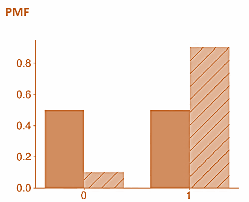
• The Bernoulli is a discrete distribution for random variables that produces one of two values: 0 or 1. It applies to any problem with a binary outcome (e.g., bull and bear markets, corporate defaults, or the classification of fraudulent transactions).
• The Bernoulli distribution depends on a single parameter, p, which is the probability that a success is observed.
• Suppose that Y is a Bernoulli random variable with parameter p. This can be expressed as
• The mean of 𝑌 is
• The Variance of 𝑌 is

  

  where

  q=1-p is the failure probability.

• The probability mass function (PMF) of a Bernoulli(p) is This function only produces two values:
  p, when y=1 and
  1-p, when y=0.
  
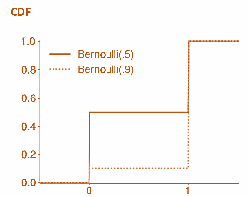
• The CDF of a Bernoulli(p) is a step function with three values:

Binomial Distribution

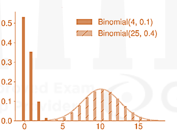
• A binomial random variable measures the total number of successes from 𝑛 independent Bernoulli random variables, where each has a probability of success equal to 𝑝. Hence, binomial distributions are used to model counts of independent events
  A binomial distribution has two parameters:
  1. n, the number of independent experiments; and
  2. p, the probability that each experiment is successful.
• If n variables are independent, then a binomial with parameters n and p is defined as

  and expressed as

  Y=B(n, p)

• The mean of a binomially distributed random variable is given by

  E[Y]=np

  The variance of 𝑌 is

  V[Y]=np(1-p)

• The skewness of a binomial depends on 𝑝, with small values producing right-skewed distributions.
• The normal distribution provides a convenient approximation to the binomial if both

  and

  

• The PMF of a B(n, p) is

  where

  

  

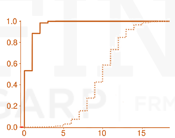
• The CDF is the sum of the cumulated PMF between 0 and y

  

• The probability that each stock will go up during an expansion is 0.80. An investor has 9 such stocks and the event of going up for any particular stock is independent of the other stocks going up. If X denote the number stocks that go up,  what is the mean, variance and standard deviation of X? What is the probability that zero, five, seven or all stocks will go up?

Poisson Distribution

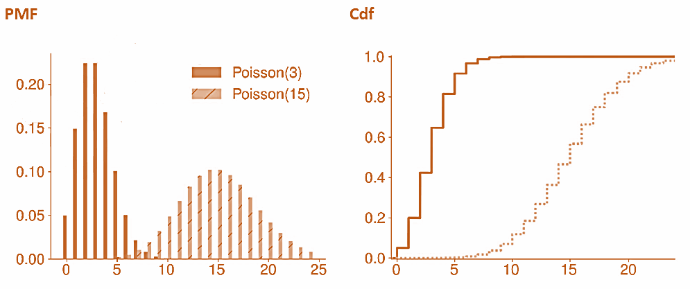
• Poisson random variables are used to measure counts of events over fixed time spans. For example, one application of a Poisson is to model the number of loan defaults that occur each month.
• Poisson random variables are always non-negative and integer-valued. The Poisson distribution has a single parameter, which is called the hazard rate and expressed as λ, that signifies the average number of events per interval.
• The mean and variance of are simply:
• If the rate at which events occur over time is constant, and the probability of any one event occurring is independent of all other events, then we say that the events follow a Poisson process, where:

  where t is the time elapsed.

• A useful feature of the Poisson (one that is uncommon among distributions) is that it is infinitely divisible.
  
  This feature makes the Poisson well-suited to work with time series data, because summing the number of events in a sampling interval (e.g., a week, month, or quarter) does not change the distribution.
• The PMF of a Poisson random variable is
• The CDF of a Poisson is defined as the sum of the PMF for values less than the input

  

• Poisson random variables are used to measure counts of events over fixed time spans. For example, one application of a Poisson is to model the number of loan defaults that occur each month.
• Poisson random variables are always non-negative and integer-valued. The Poisson distribution has a single parameter, which is called the hazard rate and expressed as λ, that signifies the average number of events per interval.The mean and variance of are simply:

  

• If the rate at which events occur over time is constant, and the probability of any one event occurring is independent of all other events, then we say that the events follow a Poisson process, where:

  where t is the time elapsed.

• A useful feature of the Poisson (one that is uncommon among distributions) is that it is infinitely divisible.
  
  are independent, and

  This feature makes the Poisson well-suited to work with timeseries data, because summing the number of events in a sampling interval (e.g., a week, month, or quarter) does not change the distribution.

Poisson Distribution – Example

If the defaults in a portfolio of bonds follow a Poisson distribution and the expected number of defaults each month is five, then find the probability that there are exactly four defaults during the next month? Also find the probability that there are exactly five defaults over the next two months?

Normal Distribution

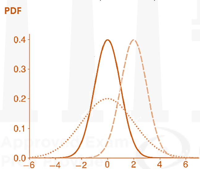
• The normal distribution is the most commonly used distribution in risk management. It is also commonly referred to as a Gaussian distribution (after Carl Friedrich Gauss) or a bell curve (which reflects the shape of the PDF). The normal distribution is popular for many reasons.
  • Many continuous random variables are approximately normally distributed.
  • The distribution of many discrete random variables can be well approximated by a normal.
  • The normal distribution plays a key role in the Central Limit Theorem (CLT), which is widely used in hypothesis testing (i.e., the process where data is used to determine the truthfulness of an objective statement).
  • Normal random variables are infinitely divisible, which makes them suitable for simulating asset prices in models that assume that prices are continuously evolving.
  • The normal is closely related to many other important distributions, including the Students’s t, the and the F
  • The normal is closed (i.e., weighted sums of normal random variables are normally distributed) under linear operations.
  • Estimators derived under the assumption that the underlying observations are normally distributed often have simple closed forms.
• It is completely described by its mean, , and variance, , stated as
• Skewness=0, thus
• Kurtosis=3. This kurtosis is often used as a benchmark when assessing whether another distribution is heavy/fat-tailed.
• The normal can generate any value in (-∞, ∞), although it is unlikely to observe values more than 3𝜎 away from the mean. In fact, values more than 3𝜎 away from the mean are expected in only one in 370 realizations of a normal random variable.
• The PDF of a normal distribution is

  

• The CDF of Y is
  
• the sums of independent normally distributed random variables are also normally distributed. If  , and

  This property simplifies describing log returns at different frequencies; if daily log returns are independent and normal, then weekly and monthly returns are as well.

• Tails get thinner and thinner and extend up to infinity.Mean=Median=Mode

Normal Distribution – Confidence Intervals

• • 68% confidence interval is μ-σ to μ+σ
  • 90% confidence interval is μ-1.645σ to μ+1.645σ
  • 95% confidence interval is μ-1.96σ to μ+1.96σ
  • 99% confidence interval is μ-2.58σ to μ+2.58σ

Example –

• The return on a stock is 12% per annum and the standard deviation of annual returns is 15%. Assuming that the returns follow a normal distribution, find the 90% confidence interval for the stock return over this year.

Standard Normal Distribution

• A standard normal distribution (or a z-distribution) is a normal distribution which has been standardized to have a mean of zero and a standard deviation of one. It is stated as X~N(0,1 )
• It is also common to use ϕ(z) to denote the standard normal PDF and Φ(z) to denote the standard normal CDF.PDF is

  

• The z-value is the number of standard deviations a given observation is away from the mean. Standardization is converting an observed value x to its z value by using the formula:

Standard Normal Distribution – Example

Consider out last example where the annual return on a stock is normally distributed with a mean of 12% per annum and a standard deviation of 15%.  Find the z-values corresponding to the returns -3% and 19.5%

Standard Normal Distribution And Probabilities

• A standard normal table, or z-table, is a mathematical table for the values of Φ, which are  values of the cumulative distribution function of the normal distribution, denoted by . By symmetry of the normal distribution
• The values in the z-table are the probabilities of observing a z-value that is less than a given value (or P[Z<z]). It can also be used to find the probability that a z-value is observed above ( by using ), or between values on the standard normal distribution, and by extension, any normal distribution.

Standard Normal Table – Example 1

Consider out last example where the annual return on a stock is normally distributed with a mean of 12% per annum and a standard deviation of 15%.  Find the probability that the return is less than or equal to 18%.

Standard Normal Table – Example 2

Consider out last example where the annual return on a stock is normally distributed with a mean of 12% per annum and a standard deviation of 15%.  Find the probability that the return is greater than 25%.

Standard Normal Table – Example 3

Consider out last example where the annual return on a stock is normally distributed with a mean of 12% per annum and a standard deviation of 15%.  Find the probability that the return is less than or equal to 2%.

Approximating Discrete Random Variables

• A normal distribution can approximate a binomial random variable if both
  np ≥ 10 and n(1 – p) ≥ 10
• When these conditions are satisfied, a binomial has either many independent experiments or a probability that is not extreme (or both), and so the PMF is nearly symmetric and well approximated by a
  N(np, np(1-p))
• The Poisson can also be approximated by a normal random variable. When λ is large, then a Poisson(λ) can be well approximated by a Normal(λ, λ). This approximation is commonly applied when λ≥1000.

Lognormal Distribution

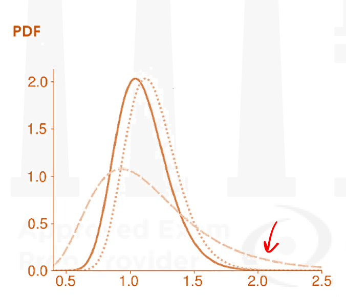
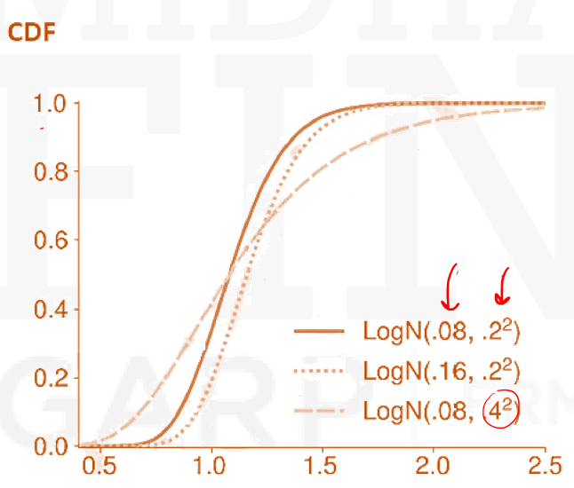
• A variable Y is said to be log-normally distributed if the natural logarithm of Y is normally distributed. In other words, if X=ln⁡ Y, then is log-normally distributed if and only if X is normally distributed. Alternatively, a log-normal can be defined where 
• An important property of the log-normal distribution is that Y can never be negative, whereas X can be negative because it is normally distributed. This log-normal property can be desirable when constructing certain models. For example, if stock prices are assumed to be normally distributed, there is a positive (although perhaps tiny) probability that the stock price becomes negative. This is impossible under a log-normal model.
• A log-normal distribution can be denoted as where ln⁡(Y) is normally distributed with mean μ and variance .
• Here, 𝑌 is a non-linear transformation of a normal random variable
• The mean of Y is
• The variance of Y is
• Lognormal distribution is positively skewed.
• It peaks at
• The PDF of a log-normal is given by:

  

• The CDF of Y is

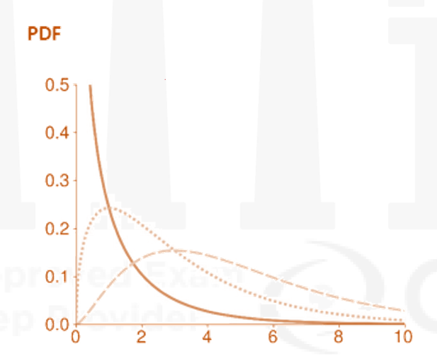
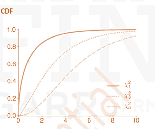
Chi Square Distribution

• • The (chi-squared) distribution is frequently encountered when testing hypotheses about model parameters. It is also used when modeling variables that are always positive, (e.g., the VIX Index).
  • A random variable is defined as the sum of the squares of ν (Greek nu) independent standard normal random variables

• Note that a distribution has 𝜈 degrees of freedom, a concept that arises when dealing with models that have 𝑘 parameters using 𝑛 data points. Degrees of freedom measure the amount of data that is available to test model parameters, because estimating model parameters requires a minimum number of observations (e.g., 𝑘). In many models, the degree of freedom used in testing is n-k.
• The mean of  is
• The variance of Y is
• The PDF of a random variable is
  

  

  where Γ(x) is known as the Gamma function.

  

• The CDF of Y is
  

  

  where P is the regularized gamma function.

  

Student’s T Distribution

• The Student’s t distribution is closely related to the normal, but it has heavier tails. It was originally developed for testing hypotheses using small samples.
• A Student’s t is a one-parameter distribution. This parameter, denoted by , is also called the degrees of freedom parameter. While it affects many aspects of the distribution, the most important effect is on the shape of the tails of the distribution.The Student’s t is the distribution of
  

  

• where
  • Z is a standard normal
  • W is a random variable, and
  • Z and W are independent.
• Dividing a standard normal by another random variable produces heavier tails than the standard normal. This is true for all values of 𝜈, although a Student’s t converges to a standard normal as ν→∞.
• If   , then the mean is

  E[Y]=0

  The mean is only finite if ν>1

• The variance of Y is

  The variance is only finite if ν>2

• The kurtosis of Y is

  The kurtosis is defined for ν>4 and is always larger than 3

• Using the basic result that

  It is easy to see that

  

  when .

  This distribution is known as a standardized Student’s t, because it has mean 0 and variance 1 for any value of ν.

• The above distribution can be rescaled to have any variance and re-centered to have any mean if ν>2. For example, is known as a generalized Student’s t and has mean μ, variance , and degrees of freedom parameter ν. It is parameterized with three parameters reflecting the mean, variance, and degrees of freedom, and is denoted as
• As compared to the normal distribution, the generalized 𝑡 is better suited to model the returns of many assets. It captures the heavy tails in asset returns while retaining the flexibility of a normal random variable to directly set the mean and variance.

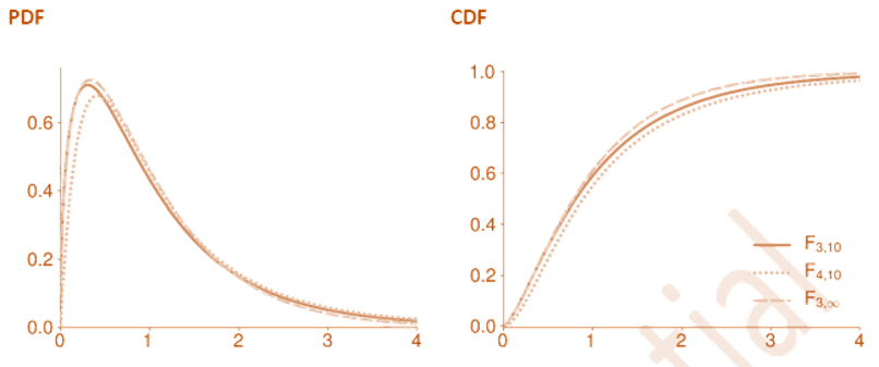
F Distribution

• The 𝐹 is another distribution that is commonly encountered when testing hypotheses about model parameters. The 𝐹 has two parameters, and
• An F distribution is defined as the ratio of two independent random variables where each has been divided by its degree of freedom

  where , and , and

  are independent.

• If , then the mean of Y is

  

  which is only finite when is larger than 2.

• The variance of Y is

  

  and is only finite for .

• When using an F in hypothesis testing, ; is usually determined by the hypothesis being tested and is typically small (e.g., 1, 2, 3, …), while is related to the sample size (and so is relatively large).
  

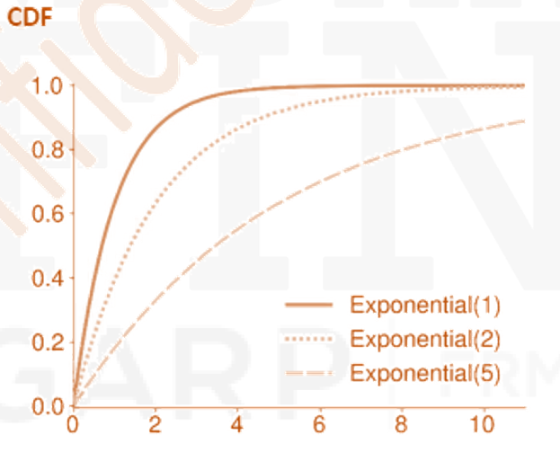
Exponential Distribution

• The exponential distribution uses a single parameter, β, that determines both the mean and variance.
• If , then mean of Y is

  E[Y]=β

• The variance of Y is

  V[Y]=β

• The exponential distribution is closely related to the Poisson distribution.
  For example, suppose X is a random variable that measures the number of loan defaults per quarter.
  If X is Poisson distributed with parameter β, then the time between each subsequent loan default has as an exponential distribution with parameter β.
• Exponential variables are also memoryless, meaning that their distributions are independent
  of their histories.
• The PDF of an Exponential(β) is

  

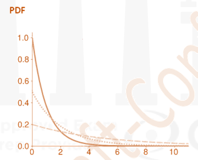
• The CDF is
  
  

Exponential Distribution Example

Assume that the time to default for a specific segment of credit card consumers is exponentially distributed with a β of 5 years. Find the probability that the customer will not default before year 6

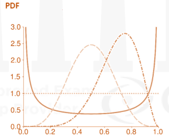
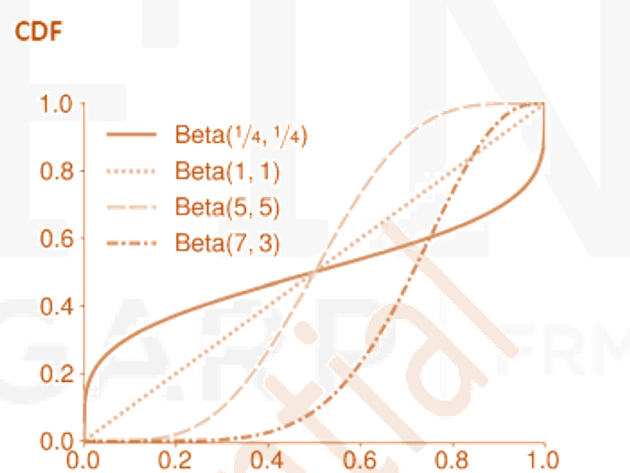
Beta Distribution

• The beta distribution applies to continuous random variables with outcomes between 0 and 1. It is commonly used to model probabilities that naturally fall into this range. The beta distribution has two parameters, α and β, that jointly determine the mean and variance of a beta-distributed random variable.
• If , then mean of Y is
• The variance of Y is
• The PDF of a beta(α, β) is

  where , and Γ(⋅) is the Gamma function.

  

• The CDF is

  where is the regularized incomplete beta function.

  

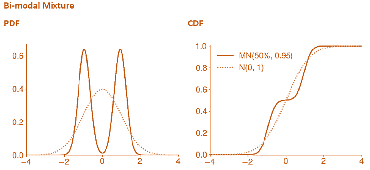
Mixtures Of Distributions

• Mixture distributions build new, complex distributions using two or more component distributions.
• A two-component mixture first draws a value from a Bernoulli random variable. Then, depending on the value (0 or 1), draws from one of two component distributions. This structure makes it simple to compute the CDF of the mixture when the components are normal random variables.
• Mixing components with different means and variances produces a distribution that is both skewed and heavy-tailed.