Introduction

• Ideally, a model should include all variables that explain the dependent variable and exclude all that do not. In practice, achieving this goal is challenging, and the model selection process must account for the costs and benefits of including additional variables.
• Once a model has been selected, the specification should be checked for any obvious deficiencies. Standard specification checks include residual diagnostics and formal statistical tests to examine whether the assumptions used to justify the OLS estimator(s) are satisfied.
• Omitted variable bias occurs when two conditions are met:

a)The omitted variable is correlated with the included independent variable.

b)The omitted variable is a determinant of the dependent variable.

• Omitting explanatory variables that affect the dependent variable creates biased coefficients. The bias depends on both the coefficient of the excluded variable and the correlation between the excluded variable and the remaining variables in the model. When a variable is excluded, the coefficients on the included variables adjust to capture the variation shared between the excluded and the included variables.
• On the other hand, including irrelevant variables does not bias coefficients. Including an unnecessary explanatory variable does, however, increase the uncertainty of the estimated model parameters.
• Determining whether a variable should be included in a model reflects a bias-variance tradeoff.  Model selection captures this bias-variance tradeoff when sample data are used to determine whether a variable should be included. Two methods are widely used to select a model from a set of candidate models: general-to-specific model selection and cross-validation.
• Once a model has been chosen, additional specification checks are used to determine whether the specification is accurate.

Omitted variables v extraneous variables

• An omitted variable is one that has a non-zero coefficient but is not included in a model. Omitting a variable has two effects –
1. First, the remaining variables absorb the effects of the omitted variable attributable to common variation. This changes the regression coefficients on the included variables so that they do not consistently estimate the effect of a change in the explanatory variable on the dependent variable (holding all other effects constant).
2. Second, the estimated residuals are larger in magnitude than the true shocks. This is because the residuals contain both the true shock and any effect of the omitted variable that cannot be captured by the included variables.
• An extraneous variable is an irrelevant variable, i.e. one that is included in the model but is not needed. This type of variable has a true coefficient of 0 and is consistently estimated to be 0 in large samples. When the true coefficient is equal to 0, RSS remains the same and the adjusted R² (denoted as R ̃² or R_a²) becomes smaller and standard error is larger.
• In most applications to financial data, correlations between the variables are large and so the impact of an extraneous variable on the standard errors of relevant variables can be substantial.

The bias-variance tradeoff

• The choice between omitting a relevant variable and including an irrelevant variable is ultimately a tradeoff between bias and variance.
1. Larger models tend to have a lower bias (due to the inclusion of additional relevant variables), but they also have less precise estimated parameters (because including extraneous variables increases estimation error).
2. On the other hand, models with few explanatory variables have less estimation error but are more likely to produce biased parameter estimates.
• The bias-variance tradeoff is the fundamental challenge in variable selection. There are many methods for choosing a final model from a set of candidate explanatory variables, and some of these methods always select the true model (at least in large samples). Other methods perform well in applications of linear regression despite having weaker theoretical foundations.
• Two of these methods are
1. general-to-specific model selection, and
2. 𝑚-fold cross-validation.

General to specific(gts) model selection

• This model selection method include following steps to select the final model from candidate models:-
1. Specify a large model that includes all relevant variables.
2. Estimate the parameters of all the variables that are included in the model.
3. Conduct a hypothesis test at 1% level of significance and if there are coefficients in this estimated model that are statistically insignificant, remove the variable with the coefficient with the smallest absolute 𝑡-statistic
4. Then, the model is re-estimated using the remaining explanatory variables. These two steps (remove and re-estimate) are repeated until the model contains no coefficients that are statistically insignificant.
5. Common choices for 𝛼 are between 1% and 0.1% (which correspond to selecting models where all absolute 𝑡-statistics are at least 2.57 or 3.29, respectively).

M-fold cross validation

• This is an alternative method that is popular in modern data science. It is designed to select a model that performs well in fitting observations not used to estimate the parameters (a process known as out-of-sample prediction).
• The steps are –
1. Cross-validation begins by randomly splitting the data into 𝑚 equal sized blocks. Common choices for 𝑚 are five and ten.
2. Parameters are then estimated using m-1 of the 𝑚 blocks, and the residuals are computed using these estimated parameter values on the data in the excluded block. Each block is used to compute residuals once. These residuals are known as out-of-sample residuals, because they are not included in the sample used to estimate parameters.
3. The sum of squared errors is then computed using the residuals estimated from the out-of-sample data.
4. Finally, the preferred model is chosen from the set of candidate models by selecting the model with the smallest out-of-sample sum of squared residuals.

In machine learning or data science applications, the m-1 blocks are referred to as the training set and the omitted block is called the validation set.

• Cross-validation selects variables with consistent predictive power and excludes variables with small coefficients that do not improve out-of-sample predictions. This mechanism has the effect of directly embedding the bias-variance tradeoff in the model selection.

Heteroskedasticity

• Homoskedasticity is one of the five assumptions used to determine the asymptotic distribution of an OLS estimator. It requires that the variance of ϵ_i is constant and so does not systematically vary with any of the explanatory variables. In models of financial data, this assumption is often false. In these cases, the residuals are heteroskedastic.
• Unconditional heteroskedasticity is when heteroskedasticity is not related with value of the independent variable, i.e. the variance of the residuals varies, but not necessarily increases or decreases with the level of the independent variable(s). Even though this is a violation of the equal variance assumption, it generally does not create any major problems with the regression.
• Conditional heteroskedasticity is when it the variance of the residuals is systematically related with the level the of independent variable(s). In the current FRM curriculum, whenever heteroskedasticity is being referred to, it is conditional heteroskedasticity.
• The effects of heteroskedasticity can be summarized as follows –
1. Regression coefficients are not affected in terms of consistency and unbiasedness, i.e. the  β_js are still consistent and unbiased.
2. The asymptotic distribution of the estimated parameters takes a different form.
3. Standard errors are usually unreliable estimates produces unreliable results.
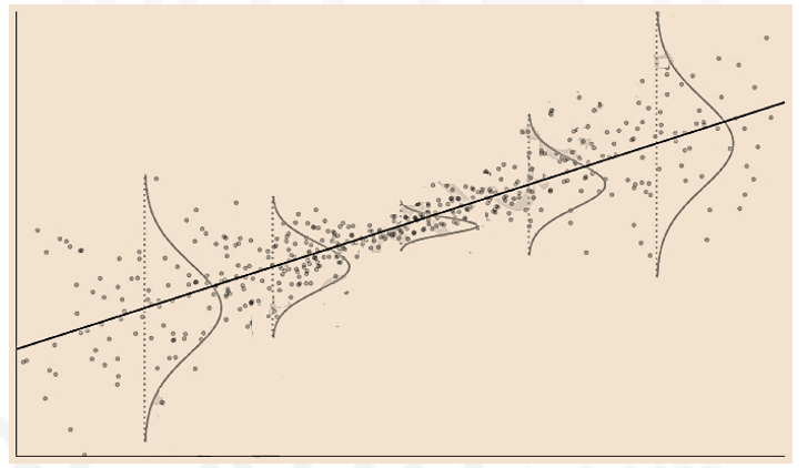
• This figure contains a simulated data set with heteroskedastic shocks. The residual variance increases as X moves away from its mean; consequently, the largest variances occur when (X-μ_X )²  is largest.This form of heteroskedasticity(i.e.,conditional) is common in financial asset returns.



• In a regression, the most extreme observations (of 𝑋) contain the most information about the slope of the regression line. When these observations are coupled with high-variance residuals, estimating the slope becomes more difficult. This is reflected by a larger standard error for β ̂.

Tests for heteroskedasticity

• When residuals are heteroskedastic, the standard errors can be estimated using White’s estimator (also called Eiker-White in some software packages). Parameters can be tested using 𝑡-tests by using White’s standard error in the place of standard error used for homoskedastic data. On the other hand, 𝐹-tests, are not as easy to adjust for heteroskedasticity and so caution is required when testing multiple hypotheses if the shocks are heteroskedastic.
• A simple test for heteroskedasticity, proposed by White is implemented as a two-step procedure.
1. Estimate the model and compute the residuals (ϵ ̂_i  ).
2. Regress the squared residuals on
3. a constant,
4. all explanatory variables, and
5. the cross product  of all explanatory variables (including the product of each variable with itself).

For example, if the original model has two explanatory variables:



then the first step computes the residuals using the OLS parameter estimators –



The second step regresses the squared residuals on a constant, X₁, X₂, X₁^², X₂^², and X₁ X₂:



• If the data are homoscedastic, then ϵ ̂_i^2 should not be explained by any the variables on the right-hand side and the null is



• The  test statistic is computed as nR², where the R² is computed in the second regression. The test statistic has a χ_(k(k+3)/2)²  distribution, where 𝑘 is the number of explanatory variables in the first-stage model.
• When k=2, the null imposes five restrictions, and the test statistic is distributed χ₅². Large values of the test statistic indicate that the null is false, so that homoscedasticity is rejected in favor of heteroskedasticity. When this occurs, heteroskedasticity-robust (White) standard errors should be used.

Approaches to modelling heteroskedastic data

• There are three common approaches used to model data with heteroskedastic shocks.
1. The first (and simplest) is to ignore the heteroskedasticity when estimating the parameters and then use the heteroskedasticity-robust (White) covariance estimator in hypothesis tests. This approach is frequently used because the parameters are estimated using OLS. However, while this method is simple, it often produces substantially less precise model parameter estimates when compared to methods that directly address heteroskedasticity.
2. The second approach is to transform the data.

For example, it is common to find heteroskedasticity in data that are strictly positive (e.g., trading volume or firm revenues). When data are always positive, it is tempting to model the natural log of the dependent variable, because it can reduce or even eliminate heteroskedasticity and may provide a better description of the data.

An alternative is to transform the data by dividing the dependent variable by another (strictly positive) variable. For example, dividing the dividend per share by the share price produces the yield of a stock. (Note that yields are often homoskedastic even when dividends per share are not.)

3. The final (and most complicated) approach is to use weighted least squares (WLS). WLS is a generalization of OLS that applies a set of weights to the data before estimating parameters. If V[ϵ_i]=w_i² σ²  and w_i  is known, then transforming the data by dividing by w_i removes the heteroskedasticity from the errors. WLS regresses Y_i/w_i   on X_i/w_i  so that:





The parameters of this model are estimated using OLS on the transformed data. The modified error is ϵ_i/w_i , and so the variance of the error (V[ϵ_i/w_i ]=σ²) is constant across observations. The challenge with implementing WLS is determining the weights.

Multicollinearity

• Multicollinearity occurs when one or more explanatory variables can be substantially explained by the other(s). For example, if a model has two explanatory variables, then the variables are multicollinear if the R² in the regression of one on the other is very high.
• Multicollinearity differs from perfect collinearity, where one of the variables is perfectly explained by the others such that the R² of a regression of X_j on the remaining explanatory variables is 1.
• Multicollinearity is a common problem in finance and risk management because many regressors are simultaneously determined by and sensitive to the same news. Multicollinearity is not ruled out by any of the assumptions of linear regression, and so it does not pose a technical challenge to parameter estimation or hypothesis testing. It does, however, create challenges in modeling data.
• The rule-of-thumb is that R² above 90% creates issues in moderate sample sizes (i.e., 100s of observations).
• When data are multicollinear, it is common to find coefficients that are jointly statistically significant (as evidenced by the 𝐹-statistic of the regression) and yet have small individual 𝑡– statistics (e.g., less than 1.96 in magnitude). This contradiction occurs because the joint statistical analysis can identify some effect from the regressors as a group (using the 𝐹-statistic) but cannot uniquely attribute the effect to a single variable (using the 𝑡-statistics).
• The above contradiction also implies that it will be common to find  R² being high (indicating joint significance), but at the same time p-values will also be high for individual coefficients (indicating individual coefficients not being significant).

Dealing with multicollinearity

• There are two options available to deal with multicollinear explanatory variables –
1. The first (and easiest) is to ignore the issue because it is technically not a problem.
2. The alternative is to identify multicollinear variables and to consider removing these from the model. The standard method to determine whether variables are excessively multicollinear is to use the variance inflation factor. This measure compares the variance of the regression coefficient on an explanatory variable X_j in two models: one that only includes X_j and one that includes all 𝑘 explanatory variables:



The variance inflation factor for variable 𝑗 is then:



where R_j² comes from a regression of X_j on the other variables in the model. Values above 10 (i.e., which indicate that 90% of the variation in X_j can be explained by the other variables in the model) are considered excessive.

Residual plots

• Residual plots are standard methods used to detect deficiencies in a model specification. An ideal model would have residuals having the following characteristics –
1. They should not systematically related to any of the included explanatory variables.
2. The residuals should also be relatively small in magnitude (i.e., typically within ±4s, where s^2 is the estimated variance of the shocks in the model).
• The basic residual plot compares ϵ ̂_i(y-axis) against the realization of the explanatory variables x_i. An alternative uses the standardized residuals ϵ ̂_i/s   so that the magnitude of the deviation is more apparent. Both outliers and model specification problems (e.g., omitted nonlinear relationships) can be detected in these plots.

Outliers

• Outliers are values that, if removed from the sample, produce large changes in the estimated coefficients.
• Cook’s distance measures the sensitivity of the fitted values in a regression to dropping a single observation 𝑗. It is defined as:



where

Y ̂_i^(-j)  is the fitted value of Y_i when observation 𝑗 is dropped and the model is estimated using 𝑛 − 1 observations,

𝑘 is the number of coefficients in the regression model, and

s² is the estimate of the error variance from the model that uses all observations.

D_j should be small when an observation is an inlier (i.e., does not disproportionately affect parameter estimates). Values of D_j larger than 1 indicate that observation 𝑗 has a large impact on the estimated model parameters.

• For example, consider the given data.

Trial 15 yields a result that is quite different from the rest of the data. To see whether this observation is an outlier, a model is fit

a)on the entire data set (i.e., Y ̂_i) as well as

b)on just the first 14 observations (i.e.,Y ̂_i^(-j)).

The resulting coefficients are





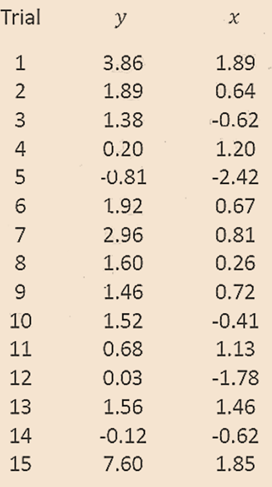
Based on the calculations which were shown in the video using excel, the variance from the full run (i.e., s^2) is calculated as 2.19 and Σ_i^n (Y ̂_i^(-j)-Y ̂_i )^2  was calculated as 4.6

Applying Cook’s distance yields



Because D_j > 1, Trial 15 can be considered an outlier.

Strengths of ols

• Under assumptions of linear regression, OLS is the Best Linear Unbiased Estimator (BLUE). Best indicates that the OLS estimator achieves the smallest variance among any estimator that is linear and unbiased.
• While BLUE is a strong argument in favor of using OLS to estimate model parameters, there are two factors which should sound alarm bells –
1. First, the BLUE property of OLS depends crucially on the homoskedasticity of the residuals. When the residuals have variances that change with 𝑋 (as is common in financial data), then it is possible to construct better LUEs of 𝛼 and 𝛽 using WLS (under some additional assumptions).
2. Second, many estimators are not linear. For example, many maximum likelihood estimators (MLEs) are nonlinear. MLEs have desirable properties and generally have the smallest asymptotic variance of any consistent estimator. MLEs are, however, generally biased in finite samples and so it is not possible to compare them to OLS in fixed sample sizes.
• If ϵ_i ∼┴iid  N(0, σ²), then OLS is the Best Unbiased Estimator (BUE). That is, the assumption that the errors are normally distributed strengthens BLUE to BUE so that OLS is the Best (in the sense of having the smallest variance) Unbiased Estimator among all linear and nonlinear estimators. This is a compelling justification for using OLS when the errors are iid normal random variables.
• However, it is not the case that OLS is only applicable when the errors are normally distributed. The only requirements on the errors are the assumptions that the residuals have conditional mean zero and that there are no outliers. Normality of the errors is not required for α ̂  and β ̂ to accurately estimate the population values or for the estimators to have desirable properties (e.g., consistency or asymptotic normality).