
Learning Objectives
- Describe the requirements for a series to be covariance-stationary.
- Define the autocovariance function and the autocorrelation function (𝐴𝐶𝐹).
- Define white noise, describe independent white noise and normal (Gaussian) white noise.
- Define and describe the properties of autoregressive (𝐴𝑅) processes.
- Define and describe the properties of moving average (𝑀𝐴) processes.
- Explain how a lag operator works.
- Explain mean reversion and calculate a mean-reverting level.
- Define and describe the properties of autoregressive moving average (𝐴𝑅𝑀𝐴) processes.
- Describe the application of 𝐴𝑅, 𝑀𝐴, and 𝐴𝑅𝑀𝐴 processes.
- Describe sample autocorrelation and partial autocorrelation.
- Describe the Box-Pierce Q-statistic and the Ljung-Box Q-statistic.
- Explain how forecasts are generated from 𝐴𝑅𝑀𝐴 models.
- Describe the role of mean reversion in long-horizon forecasts.
- Explain how seasonality is modeled in a covariance-stationary 𝐴𝑅𝑀𝐴.
- Video Lecture
- |
- PDFs
- |
- List of chapters
Chapter Contents
- Introduction
- Stochastic Processes
- Covariance Stationary
- Autocovariance
- Autocorrelation and partial autocorrelation
- White noise
- White noise – world’s theorem
- Dependent white noise
- Autoregressive (AR) models
- Autoregressive models – AR(p)
- The lag operator
- Moving average (MA) models
- Moving average models – MA(q)
- Mean reversion and mean reverting level
- Autoregressive moving average models
- Autoregressive moving average models – ARMA(p,q)
- Sample autocorrelation
- Testing autocorrelations – graphical inspection
- Testing autocorrelations – joint tests
- Sample autocorrelation – joints tests
- Parameter estimation in AR and ARMA models
- Model selection
- Model selection – Box-jenkins methodology
- Forecasting
- Forecasting – the mean reverting level
- Seasonality
Introduction
- Time-series analysis is a fundamental tool in finance and risk management. Many key time series (e.g., interest rates and spreads) have predictable components. Building accurate models allows past values to be used to forecast future changes in these series.
- A time series can be decomposed into three distinct components –
- The trend – It captures the changes in the level of the time series over time.
- The seasonal component – It captures predictable changes in the time series according to the time of year.
- The cyclical component – It captures the cycles in the data.
- The first two components are deterministic (components evolve in a perfectly predictable way), and the third component is determined by both the shocks to the process and the memory (i.e., persistence) of the process.
Stochastic Processes
- Stochastic processes are ordered collections of random variables. They are denoted using {Yt}, reflecting the fact that they are sequences of random variables that are ordered in time (t) (i.e., Ys is observed before Yt whenever s<t). The ordering of a time series is important when predicting future values using past observations.
- One of the simplest and useful stochastic processes is
- Any linear process can be written as –
- Linear processes are important for two reasons –
- First, a wide range of processes, even nonlinear processes, have linear representations.
- Second, linear processes can be directly related to linear models, which are the workhorses of time-series analysis.
This process is linear in {ϵt}, which is a mean zero stochastic process commonly referred to as the shock. The process δt is deterministic and coefficients on the shocks, ψis, are constant.
Covariance Stationary
- The ability of a model to forecast a time series depends crucially on whether the past resembles the future. To forecast a series, at least its mean and its covariance structure (i.e., the covariances between current and past values) should be stable over time, or in other words, the series should be covariance stationary. A time series is covariance-stationary if –
- The mean is constant and does not change over time (E[Yt] = μ for all t).
- The variance is finite and does not change over time (V[Yt] = γ_0< ∞ for all t).
- The autocovariance is finite, does not change over time, and only depends on the distance between the observations (ℎ) (Cov[Yt, Y(t-h) ] = γh for all t).
- Covariance stationarity is important when modeling and forecasting time series because of –
- Constant relationships – A covariance-stationary time series has constant relationships across time. It allows historical data to be used to estimate models that are applicable to future, out-of-sample observation.
- Parameter estimation and interpretation – Stationary time series are easy to interpret because their estimated parameters are asymptotically normally distributed. Furthermore, stationary time series do not suffer from spurious relationships where unrelated series appear to have strong, statistically significant correlations.
Autocovariance
- Autocovariance is defined as the covariance between a stochastic process at different points in time. Its definition is the timeseries analog of the covariance between two random variables. The h^th autocovariance is defined as –
- If the covariance structure is stable over time, as required by covariance stationarity, then the autocovariances depend only on displacement, h, and not on time, t, such that –
- The autocovariance function is symmetric, that is –
- When h=0, then γ(t,0) = E[(Yt-E[Yt ])2 ]. This is the variance of Yt.
where
the subscripts denote the period (i.e., t) and the lag (i.e., h) between observations.
Symmetry reflects the fact that the autocovariance of a covariance stationary series depends only on displacement. It doesn’t matter whether the movement is forward or backward.
Autocorrelation and partial autocorrelation
- If {Y_t} is covariance-stationary, the autocorrelation is defined as the ratio –
- Autocorrelations, like correlations, are always between -1 and 1 (both inclusive).
- The autocorrelation function (ACF) is similarly defined using the autocorrelations as
- The partial autocorrelation function (PACF) measures the strength of the correlation between Yt and Y(t-h) after controlling for the values between them (i.e.,Y(t-1),Y(t-2),…Y(t-h+1)).
- Partial autocorrelation is a nonlinear transformation of the ACF and is widely used in model selection. It is identical to the autocorrelation at the first lag as there are no values between Yt and Y(t-1) , but it differs at all other lags. This function is commonly represented as α(h).
ρ(h) = ρ_|h|
White noise
- White noise is the fundamental building block of any time-series model. A white noise process is denoted as –
- White noise processes {ϵ_t} have three properties –
- Mean zero (E[ϵ_t ]=0)
- Constant and finite variance (V[ϵt ]=σ2 < ∞)
- No autocorrelation or autocovariance (Cov[ϵt,ϵ(t-h) ]=0 for all h≠0)
- Independent and identically distributed (iid) random variables are a special case of a white noise process. Any iid sequence that has mean zero and finite variance is white noise.
- Gaussian white noise is a special case of iid noise. It is represented as –
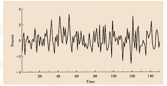
- This figure shows a simulated sample path of Gaussian white noise, of length T=150. There are no patterns of any kind in the series due to the independence over time.
- The unconditional mean and variance of white noise, yt~WN(0, σ^2 ) are constant.
- The unconditional mean of y is E(yt )=0
- The unconditional variance of y is Var(yt )=σ^2
- The autocorrelation function for a white noise process is –
- The partial autocorrelation function of a white noise process is –
where
σ2 is the variance of the shock.
White noise is uncorrelated over time so, all the autocovariances and all the autocorrelations are 0 beyond displacement 0. The autocovariance function for a white noise process is –
White noise – world’s theorem
- World’s theorem establishes the key role of white noise in any covariance-stationary process. It also provides an important justification for using linear processes to model covariance-stationary time series.
- If {Y_t} is a mean-zero covariance-stationary process, then –
- World’s theorem also states that this representation of a covariance-stationary process is unique.
where
ψ0, ψ1, … are constants,
{ϵt} is a white noise process,
ψ0 = 1, and
Dependent white noise
- Dependent white noise is particularly important in finance and risk management because asset returns are unpredictable but have persistent time-varying volatility. It relaxes the iid assumption while maintaining the three properties of white noise.
- A leading example of a dependent white noise process is known as an Autoregressive Conditional Heteroskedasticity (ARCH) process. The variance of a shock from an ARCH process depends on the magnitude of the previous shock. This process exhibits a property called volatility clustering, where volatility can be above or below its long-run level for many consecutive periods.
- Volatility clustering is an important feature of many financial time series, especially asset returns. The dependence in an ARCH process leads it to have a predictable variance but not a predictable mean, and shocks from an ARCH process are not correlated across time.
Autoregressive (AR) models
- Autoregressive (AR) models are the most widely applied time-series models in finance and economics. These models relate the current value of a stochastic process (i.e., Y_t) to its previous value (i.e., Y_(t-1)). For example, an AR(1)evolves according to –
- The AR parameter determines the persistence of 𝑌. This means that an AR(1) process is covariance-stationary when |ϕ| < 1 and non-stationary when ϕ=1.
- Since, {Yt} is assumed to be covariance-stationary, the mean, variance, and autocovariances are all constant. Using the property of a covariance-stationary time series that E[Yt ]=E[Y(t-1) ]=μ,
the long-run (or unconditional) mean of the above AR(1) is – - The variance is –
- The first autocovariance is in the AR(1) process is
- The remaining autocovariances can be recursively computed as –
- The autocovariance function is then calculated as – γ(h)=ϕ^|h| γ0
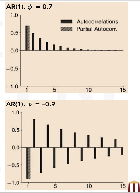
- The ACF geometrically decays to zero as ℎ increases. It also oscillates between negative and positive values if -1<ϕ<0. In practice, negative values of 𝜙 are uncommon in economic and financial time series.
- The PACF of an AR(1) is –
- The PACF is non-zero only for the first lag. The general patterns (slow decay in the ACF and a steep cutoff in the PACF) play a key role when choosing appropriate models to apply to a data set.
- The top panel in this figure shows the ACF and PACF of an AR(1) process when ϕ=0.7. The bottom panel shows the ACF and PACF when ϕ is negative (ϕ=-0.9).
- The pth order AR process generalizes the first-order process. The AR(p) model is given as –
- Deriving the properties for an AR(p) model is more involved than for an AR(1) but the properties of an AR(p) broadly mirror those of an AR(1).
- When {Yt} is covariance-stationary, the long-run mean is –
- The autocorrelation and PACFs of an AR(p) share a common structure with the ACF and PACF of an AR(1).
- The lag operator (L) is a convenient tool for expressing and manipulating more complex time series models. It shifts the time index of an observation, so that LYt=Y_(t-1).
- Six properties of lag operator are –
- The lag operator shifts the time index back one observation, (LYt=Y(t-1))
- Lp Yt=Y(t-p), for example L2 Yt=L(LYt )=LY_(t-1)=Y(t-2)
- The lag operator applied to a constant is just the constant (Lδ=δ)
- The p^th order lag polynomial is written as –
- Lag polynomials can be multiplied. For example, if a(L) and b(L) are first-order polynomials, then:
- If the coefficients in the lag polynomial satisfy some technical conditions, the polynomial can be inverted so that a(L)a(L)-1 = 1. A first-order polynomial a(L) expressed as (1 – a1 L), is invertible if |a_1 |<1 and its inverse is –
- The concept of invertibility is useful for two reasons –
- A first-order moving average model, denoted as MA(1), is defined as –
- When θ is positive, an MA(1) is persistent because two consecutive values are (on average) positively correlated. When θ is negative, the process aggressively mean reverts because the effect of the previous shock is reversed in the current period.
- Moving averages are always covariance-stationary. An MA(1) has a limited memory, because only the shock in the previous period impacts the current value.
- The mean of the MA(1) process is E[Yt ]=μ and the variance of is V[Yt ]=(1+θ2 ) σ2 .
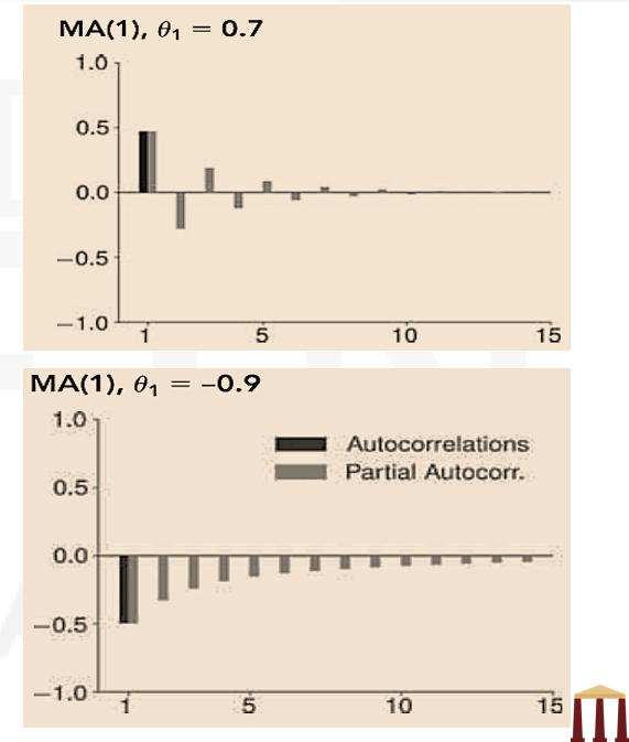
- Any MA(1) has exactly one non-zero autocorrelation, and the ACF is –
- The PACF of an MA(1) is complex and has non-zero values at all lags. This pattern is the inverse of what an AR(1) would produce.
- The upper panel in this figure shows the autocorrelation and PACF of a MA(1) process which has a positive coefficient. The lower panel shows the autocorrelation and PACF of a MA(1) process which has a negative coefficient.
- MA(1) can be generalized to MA(q), which includes q lags of the shock. It is expressed as –
- The variance of an MA(q) can be shown as –
- The autocovariance function is given as –
- In general, the ACF is always zero for lags larger than 𝑞 and the PACF is non-zero at all lags.
- A time series is mean reverting if it tends to fall when its level is above its long-run mean and rise when its level is below its long-run mean. If a time series is covariance stationary, then it will be mean reverting.
- For an AR(1) process, the mean reverting level is –
- If the MA process has an intercept term (μ), then this intercept term, μ, is the mean reverting level for both MA(1) as well as MA(q) processes. If there are no intercept, then the mean reverting level for both MA(1) and MA(q) processes is 0.
- Autoregressive Moving Average (ARMA) processes combine AR and MA processes. A simple ARMA(1,1) process evolves according to –
- The mean (μ) and variance (γ_0 ) of this process is given as –
- The autocovariance function is complicated, even in an ARMA(1,1). It can be shown as –
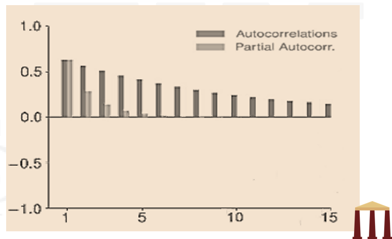
- The ACF decays as h increases and oscillates if ϕ<0. This is consistent with the ACF of an AR process. The PACF also slowly decays toward zero as the lag length increases. This behavior is consistent with a MA process.
- The slow decay of both the PACF and ACF is the key feature that distinguishes an ARMA from an AR or an MA process.
- This figure shows the autocorrelation and PACF of an ARMA(1,1) process with ϕ=0.80 and θ=-0.40.
- ARMA(p, q) processes combine AR(p) and MA(q) processes to produce models with more complicated dynamics. An ARMA(p, q) evolves according to –
- Using lag polynomials, it can be expressed as –
- Like ARMA(1,1), the ARMA(p, q) is covariance-stationary if the AR component is covariance-stationary. The autocovariance and ACF of ARMA processes are more complicated than pure AR or MA models, although the general pattern in these is simple. ARMA(p, q) models have ACFs and PACFs that decay slowly to zero as the lag increases (while possibly oscillating).
- Sample autocorrelation and partial autocorrelations are used to build and validate ARMA models. The most common estimator of the sample autocovariance is –
- The autocorrelation estimator is then defined as –
- The autocorrelation estimator has a slight bias towards zero that disappears as T becomes large.
- Testing autocorrelation in the residuals is a standard specification check applied after fitting an ARMA model. It is common practice to use both graphical inspections as well as formal tests in specification analysis.
- Graphical examination of a fitted model includes plotting the residuals to check for any apparent deficiencies and plotting the sample ACF and PACF of the residuals (i.e., ϵ ̂t ). But relying solely on graphical examination can be misleading, because it is common to see a few estimates outside of the 95% confidence bands, even in a well-specified model.
- Two closely related joint tests of autocorrelations are often used when validating a model. These are –
- The Box-Pierce test statistic
- The Ljung-Box test statistic
- Both test the joint null hypothesis that, all the autocorrelations are simultaneously zero
- Both tests have asymptotic χh2 distributions. Values of the test statistic larger than the critical value indicate that the autocorrelations are not zero.
- The Box-Pierce test statistic is the sum of the squared autocorrelations scaled by the sample size T. It is defined as –
- The Ljung-Box test statistic is a version of the Box-Pierce statistic that works better in smaller samples. It is defined as –
- In large samples QBP ≈ QLB . When T is modest (e.g., 100), the finite sample distribution of the Ljung-Box (when the null is true) is closer to the asymptotic χh2 distribution. Therefore, it is the preferred method to test multiple autocorrelations.
- The choice of ℎ can affect the conclusion of the test that the residuals have no autocorrelation. When testing the specification of an ARMA(p,q) model, ℎ should be larger than max(p,q). It is common to use between 5 and 20 lags when testing a small ARMA model (p,q≤2).
- Numerical examples based on joint tests have been solved in the video.
- The parameters of an AR(p) model can be estimated using OLS. The dependent variable is Yt and the explanatory variables are the 𝑝 lagged values.
- Estimation of the parameters in an AR is identical to parameter estimation in linear regression models. Standard errors are also estimated using the same expressions as in a linear regression. Whereas, the linear regression parameter estimators are unbiased, parameter estimators of the AR coefficients are biased (although they are consistent).
- OLS cannot be used when an MA component is added to an AR or when estimating a pure MA. This is because, OLS requires that all explanatory variables are observable, the lagged errors that appear on the right-hand side of an MA do not meet this requirement and can only be inferred once the model parameters have been estimated. The coefficients of MA and ARMA models are instead estimated using maximum likelihood, which assumes that the innovations are jointly normally distributed with mean zero and variance σ^2.
- The first step in model building is to inspect the sample autocorrelation and PACFs for essential insights into the correlation structure of the data. This inspection helps to determine the class of models that are likely to explain that structure. Slow decay in the sample ACF indicates that the model needs an AR component, and slow decay in the sample PACF indicates that the model should have an MA component.
- The next step is to measure their fit. The most natural measure of fit is the sample variance of the estimated residuals (Mean Squared Error) of the model. It is defined as –
- Choosing a model to minimize the residual variance σ ̂^2 also selects a specification that is far too large. This problem is same as the increase in R^2 leading to ovefitting in a linear regression if new variables are added. The solution to this problem is to add a penalty to the MSE that increases each time a new parameter is added. Penalized MSE measures are known as information criteria (IC). Two leading IC are –
- Akaike Information Criterion (AIC)
- Bayesian Information Criterion (BIC)/Schwarz Information Criteria (SIC)
- These IC reflect the bias-variance tradeoff and attempt to balance the cost and benefit of alternative specifications that include different orders of the AR and MA components. The AIC and BIC are defined as –
- It is important to note that the penalty term in the AIC adds a constant “cost” of two per parameter, whereas the penalty in the BIC has a cost that slowly increases with 𝑇. This difference in the penalty has two implications –
- The BIC always selects a model that is no larger than the model selected by the AIC.
- The BIC is a consistent model selection criterion (the true model is selected as 𝑇 → ∞).
- The difference between the two IC, in the context of hypothesis testing are –
- The AIC behaves like a model selection methodology that includes any variable that is statistically significant with a fixed-test size of s%. When using a fixed-test size, there is an s% chance that a coefficient that is not relevant is selected. In aggregate, this can lead to selecting models that are too large.
- he BIC behaves like AIC, but s→0 as T→∞. The quantity s goes to 0 slowly, so that any relevant variable always has a 𝑡-statistic that is larger than the required critical value in large samples. Variables that are not needed, always have 𝑡-statistics that are less than the critical value. As a result, such variables are always excluded.
- It is possible that two (or more) models that have different parameter values, have the same mean, ACF, and PACF. The Box-Jenkins methodology provides two principles to select a model among equivalent models. These principles are –
- Parsimony – When selecting between models that are equivalent (and thus produce the same fit), the model with fewer parameters should always be chosen.
- Invertibility – When choosing parameters in MA processes (either pure MA or ARMA), parameter values should be selected such that the MA coefficients are invertible.
- Using current information to predict the future is termed as forecasting. It is common to make one-step-ahead forecasts, but forecasts can be generated for any horizon ℎ.
- The one-step forecast E[Y(T+1) |FT] (or ET [Y(T+1) ] using the shorthand notation) is the expectation of Y(T+1) conditional on FT (time information set). FT contains all values that are known at time T, including the entire history of Y (YT,Y(T-1)…..). It also includes the history of the shocks (ϵT,ϵT-1…..) as well as all values of any other variable that occurred at time T or earlier.
- Three rules that simplify recursively generating forecasts are –
- The expectation of any variable with a time subscript 𝑇 or earlier is the realization of that variable, e.g. ET [YT]=YT. This is also true for residuals (ET [ϵ_(T-2)]=ϵ_(T-2)).
- The expectation of future shocks is zero (e.g. ET [ϵ(T+1)] = 0).
- Forecasts are generated recursively, starting with E_T [Y_(T+1 )]. The forecast at horizon ℎ may depend on forecasts from earlier steps –
- Applying these rules to an AR(1), the one-step forecast will be –
- Similarly, the two-step ahead forecast will be –
- These steps can be repeated for any horizon h so that:
- Steps used for AR process can be used to generalize MA and ARMA processes using the three rules of forecasting. For example,
- The forecast error is the difference between the realized (future) value and its time T forecast and is defined as Y(T+h) – ET [YT+h ]. The one-step forecast error is –
- Forecasts errors for longer-horizon forecasts are mostly functions of the model parameters.
- In an AR process, when ℎ is large, ϕ^h must be small because {Y_t} is assumed to be a stationary time series. It can be shown that –
- This duality between the mean reversion level and the long run-forecast reflects a property of any covariance-stationary time series – “the current value of Y_T always has a negligible impact on the values of 𝑌 in the distant future”. Formally, in any covariance-stationary time series:
- MA processes depend on (at most) 𝑞 lags of the residual, and so all forecasts for horizon h>q are the long-run mean μ.
- Macro-financial time series often have seasonality. It can be deterministic or stochastic. Series with deterministic seasonality are non-stationary, whereas those with stochastic seasonality can be stationary. Seasonality occurs on an annual basis. For example, the seasonal component for quarterly data appears in gaps of 4 and that of monthly data appears in gaps of 12.
- A pure seasonal model only uses lags at the seasonal frequency. For example, a pure seasonal AR(1) model of quarterly data series is
- A more plausible structure includes both short-term and seasonal components. The seasonal component uses lags at the seasonal frequency, while the short-term component uses lags at the observation frequency. A seasonal ARMA combines these two components into a single specification. For example, a model using monthly data with a seasonal AR(1) and a short-term AR(1) is –
- Seasonality can be introduced to the AR component, the MA component, or both. This is done by multiplying the short-run lag polynomial by a seasonal lag polynomial. The specification of Seasonal ARMA models is denoted as –
- In practice, seasonal components are usually restricted to one lag because the precision of the parameters related to the seasonal component depends on the number of full seasonal cycles in the sample.
where
δ is called the intercept,
ϕ is the AR parameter, and
ϵt ∼ WN(0,σ2) is the shock.
The variance of Yt depends on both the variance of the shocks (i.e., σ2) and the AR parameter (i.e., ϕ). This formula relies on the white noise assumption for ϵ_t, that Cov[Y(t-1),ϵ_t] is zero because Y(t-1) is uncorrelated with ϵ(t-1),ϵ(t-2),….
Applying the recursion, γ2 = ϕγ1 = ϕ2 γ0, and (in general) –
γh = ϕh γ0
And the ACF is –
Autoregressive models – AR(p)
And the long-run variance is
The lag operator
For example –
or,
Polynomial multiplication is commutative so that a(L)b(L) = b(L)a(L).
a)First, an AR process is only covariance-stationary if its lag polynomial is invertible.
b)Second, invertibility plays a key role when selecting a unique model for a time series using the Box-Jenkins methodology.
Moving average (MA) models
where,
ϵt ~ WN(0,σ^2) is a white noise process,
ϵt is the current shock,
ϵt-1 is the previous shock and
θ is determines the strength of effect of previous shock.
Moving average models – MA(q)
where, μ is the mean of Yt because all shocks are white noise and so have zero expected value.
where θ0 = 1
Mean reversion and mean reverting level
And the mean reverting level for an AR(p) process is –
Autoregressive moving average models
Autoregressive moving average models – ARMA(p,q)
Sample autocorrelation
where
Y ̅ is the full sample average.
This estimator uses all available data to estimate γ ̂h.
Testing autocorrelations – graphical inspection
Testing autocorrelations – joint tests
versus
the alternative hypothesis that at least one is non-zero
When the null is true, the test statistic is distributed as a χh2.
The Ljung-Box test is also distributed as a χh2.
Sample autocorrelation – joints tests
Parameter estimation in AR and ARMA models
Model selection
Smaller values indicate that the model explains more of the time series.
where
𝑇 is the sample size and
𝑘 is the number of parameters.
Model selection – Box-jenkins methodology
These two principles are enough to ensure that a unique specification is selected to match any ACF and PACF.
Forecasting
This is true for any horizon h, i.e. ET [ϵ(T+h)] = 0
One-step ahead forecast depends only on the final observed value YT.
The two-step forecast depends on the one-step forecast. So, it is also a function of YT .
suppose an MA(2) is represented as –
The first three forecasts will be –
Forecasting – the mean reverting level
This limit is the same as the mean reversion level (or long-run mean) of an AR(1).
which is the long-run (or unconditional) mean.
Seasonality
However, this structure is not plausible in most economic time series.
where
p and q are the orders of the short-run lag polynomials,
p_s and q_s are the orders of the seasonal lag polynomials, and
f is the seasonal horizon (e.g., 4 or 12).
For example, the seasonal AR in the example discussed is an ARMA(1,0)×(1,0)12
Go to Syllabus
Courses Offered
Popular Courses
FRM Part 1
FRM Part 2

By : Micky Midha
9 Hrs of Videos
Available On Web, IOS & Android
Access Until You Pass
Lecture PDFs
Class Notes

By : Micky Midha
12 Hrs of Videos
Available On Web, IOS & Android
Access Until You Pass
Lecture PDFs
Class Notes

By : Micky Midha
257 Hrs Of Videos
Available On Web, IOS & Android
Access Until You Pass
Complete Study Material
Quizzes,Question Bank & Mock tests

By : Micky Midha
240 Hrs Of Videos
Available On Web, IOS & Android
Access Until You Pass
Complete Study Material
Quizzes,Question Bank & Mock tests

By : Shubham Swaraj
Lecture Videos
Available On Web, IOS & Android
Complete Study Material
Question Bank & Lecture PDFs
Doubt-Solving Forum