
Learning Objectives
- Estimate the mean, variance, and standard deviation using sample data.
- Explain the difference between a population moment and a sample moment.
- Distinguish between an estimator and an estimate.
- Describe the bias of an estimator and explain what the bias measures.
- Explain what is meant by the statement that the mean estimator is BLUE.
- Describe the consistency of an estimator and explain the usefulness of this concept.
- Explain how the Law of Large Numbers (LLN) and Central Limit Theorem (CLT) apply to the sample mean.
- Estimate and interpret the skewness and kurtosis of a random variable.
- Use sample data to estimate quantiles, including the median.
- Estimate the mean of two variables and apply the CLT.
- Estimate the covariance and correlation between two random variables.
- Explain how coskewness and cokurtosis are related to skewness and kurtosis.
- Video Lecture
- |
- PDFs
- |
- List of chapters
Chapter Contents
- Estimating The Mean
- The First two Moments
- Bias of the Mean
- Estimating The Variance And Standard Deviation
- The First Two Moments
- The Median and Other Quantiles
- Covariance and Correlation
- Multivariate Moments
- Sample Mean of Two Variables
- Multivariate Moments
- Coskewness and Cokurtosis
- Multivariate Moments
- Standard Errors Versus Standard Deviation
- Presenting The Mean and Standard Deviation
- Scaling of the Mean and Standard deviation
- Estimating the Mean and Variance using Data
- Higher Moments
- Histograms and Kneel Destiny Plots
- The Blue Mean Estimator
- Large Sample Behavior of the Mean
- Central Limit Theorem
- Large Sample Behavior of the Mean
- The Median and Other Quantiles
- Covariance and Correlation
- Multivariate Moments
- Sample Mean of Two Variables
- Multivariate Moments
- Coskewness and Cokurtosis
- Multivariate Moments
Estimating The Mean
- The mean estimator is defined as:
- The random variables Xi are assumed to be independent and identically distributed, so that E[Xi]=μ and V[Xi]=σ2 for all 𝑖.
- An estimator is a function or a mathematical procedure that calculates an estimate based on an observed data set. In contrast, an estimate is the value produced by an application of the estimator to data.
- The mean estimator is a function of random variables, and so it is also a random variable.
The First two Moments
- The expected value of the mean estimator is the same as the population mean μ whenever the mean is constant (i.e., 〖E[Xi]=μ for all i).
Bias of the Mean
- The bias of an estimator is defined as:
- The general formula for the variance of a sum is the sum of the variances plus any covariances between the random variables:
Estimating The Variance And Standard Deviation
- Given a set of n iid random variables Xi , the sample estimator of the variance is
The First Two Moments
- Unlike the mean, the sample variance is a biased estimator. It can be shown that:
- The sample variance is therefore biased with:
- The bias arises because the sample variance depends on the estimator of the mean. Estimation of the mean consumes a degree of freedom, and the sample mean tends to resemble the sample of data a little too well (especially for smaller sample sizes). This slight “overfitting” of the observed data produces a slight underestimation of the population variance.
- Because the bias is known, an unbiased estimator for the variance can be constructed as:
- This estimator is unbiased, as E[s2] = σ2. This expression for the mean shows that (in large samples) the distribution of the sample mean estimator (μ ̂) is centered on the population mean (μ), and the variance of the sample average declines as n grows.
The Median and Other Quantiles
- The median, like the mean, measures the central tendency of a distribution. Specifically, it is the 50% quantile of the distribution and the point where the probabilities of observing a value above or below it are equal (i.e., 50%).
- When a distribution is symmetric, the median is in the center of the distribution and is the same as the mean.
- When distributions are asymmetric, the median is larger (smaller) than the mean if the distribution is left-skewed (right-skewed).
- Estimation of the median is simple. First, the data are sorted from smallest to largest.
- When the sample size is odd, the value in position (n + 1)/2 of the sorted list is used to estimate the median:
- When the sample size is even, the median is estimated using the average of the two central points of the sorted list:
- Two other commonly reported quantiles are the 25% and 75% quantiles. These are estimated using the same method as the median.
- More generally, the α-quantile is estimated from the sorted data using the value in location 𝛼𝑛. When 𝛼𝑛 is not an integer value, then the usual practice is to take the average of the points immediately above and below αn.
- These two quantile estimates (q ̂_25and q ̂_75) are frequently used together to estimate the interquartile range:
- The IQR is a measure of dispersion and so is an alternative to standard deviation. Other quantile measures can be constructed to measure the extent to which the series is asymmetric or to estimate the heaviness of the tails.
- Two features make quantiles attractive.
- First, quantiles have the same units as the underlying data, and so they are easy to interpret. For example, the 25% quantile for a sample of asset returns estimates the point where there is 25% probability of observing a smaller return (and a 75% probability of observing a larger return). Meanwhile, the interquartile range estimates a central interval where there is 50% probability of observing a return.
- Second, quantiles are robustness to outliers. For example, suppose that some observed data {x1, … , xn} are contaminated with an outlier. Both the median and IQR are unaffected by the presence of an outlier. However, this is not true of the mean estimator, which gives weight 1/n to the outlier. If the outlier is far from the other (valid) observations, this distortion can be large. The variance, because it squares the difference between the outlier and the mean, is even more sensitive to outliers.
| Daily Data | ||||
| Bonds | Stocks | Gold | Crude | |
| Median | 0.034% | 0.103% | 0.014% | 0.058% |
| q(.25) | -0.140% | -0.534% | -0.445% | -1.21% |
| q(.75) | 0.207% | 0.660% | 0.496% | 1.30% |
| IQR | 0.347% | 1.19% | 0.941% | 2.51% |
| Weekly Data | ||||
| Bonds | Stocks | Gold | Crude | |
| Median | 0.159% | 0.459% | 0.044% | 0.224% |
| q(.25) | -0.244% | -1.12% | -1.01% | -2.64% |
| q(.75) | 0.542% | 1.69% | 1.24% | 3.03% |
| IQR | 0.786% | 2.81% | 2.24% | 5.67% |
| Monthly Data | ||||
| Bonds | Stocks | Gold | Crude | |
| Median | 0.640% | 1.56% | 0.265% | 0.839% |
| q(.25) | -0.220% | -2.47% | -2.29% | -5.14% |
| q(.75) | 1.42% | 4.12% | 2.84% | 6.72% |
| IQR | 1.64% | 6.59% | 5.14% | 11.9% |
Covariance and Correlation
- Covariance measures the linear dependence between two random variables and is defined as:
- The sample covariance estimator uses the sample analog to the expectation operator
Multivariate Moments
- Correlation is the standardized version of the covariance and is usually preferred because it does not depend on the scale of X or Y. The correlation is estimated by dividing the sample covariance by the product of the sample standard deviations of each asset:
- The sample correlation estimator is biased in finite samples, even if unbiased estimators are used to estimate the variances and covariance.
| Daily Data | ||||
| Bonds | Stocks | Gold | Crude | |
| Bonds | — | -16.4% | 3.0% | -9.9% |
| Stocks | -16.4% | — | -2.1% | 12.5% |
| Gold | 3.0% | -2.1% | — | 13.0% |
| Crude | -9.9% | 12.5% | 13.0% | — |
| Weekly Data | ||||
| Bonds | Stocks | Gold | Crude | |
| Bonds | — | -2.4% | 2.3% | -7.7% |
| Stocks | -2.4% | — | 4.0% | 13.2% |
| Gold | 2.3% | 4.0% | — | 15.2% |
| Crude | -7.7% | 13.2% | 15.2% | — |
| Monthly Data | ||||
| Bonds | Stocks | Gold | Crude | |
| Bonds | — | 15.1% | 19.6% | -0.2% |
| Stocks | 15.1% | — | -0.2% | 11.6% |
| Gold | 19.6% | -0.2% | — | 18.9% |
| Crude | -0.2% | 11.6% | 18.9% | — |
Sample Mean of Two Variables
- Estimating the means of two random variables is no different from estimating the mean of each separately, so that:
- When data are iid, the CLT applies to each estimator. However, it is more useful to consider the joint behavior of the two mean estimators by treating them as a bivariate statistic. The CLT can be applied by stacking the two mean estimators into a vector:
Multivariate Moments
- The CLT for the vector depends on the 2-by-2 covariance matrix for the data. The CLT for a pair of mean estimators is virtually identical to that of a single mean estimator, where the scalar variance is replaced by the covariance matrix. The CLT for bivariate iid data series states that:
- In practice, this CLT is applied by treating the mean estimators as a bivariate normal random variable:
- Applying the bivariate CLT:
- The most important insight from the bivariate CLT is that correlation in the data produces a correlation between the sample means. Moreover, the correlation between the means is identical to the correlation between the data series.
| Moment | μ̂_X | σ_S^2 | μ̂_X | σ_B^2 | σ_SB | ρ |
| 10.4 | 335.4 | 6.71 | 25.6 | 14.0 | 0.151 |
Coskewness and Cokurtosis
- Like variance, skewness and kurtosis can be extended to pairs of random variables. When computing cross pth moments, there are p-1 different measures. Applying the principle to the first four moments there are
- No cross means,
- One cross variance (covariance),
- Two measures of cross-skewness (coskewness), and
- Three cross-kurtoses (cokurtosis).
- The two coskewness measures are
- The coskewness standardizes the cross-third moments by the variance of one of the variables and the standard deviation of the other, and so is scale- and unit-free.
- These measures both capture the likelihood of the data taking a large directional value whenever the other variable is large in magnitude. When there is no sensitivity to the direction of one variable to the magnitude of the other, the two coskewnesses are 0. For example, the coskewness in a bivariate normal is always 0, even when the correlation is different from 0.
- The univariate skewness estimators are s(X, X, X) and s(Y, Y, Y).
Multivariate Moments
- Coskewnesses are estimated by applying the sample analog to the expectation operator to the definition of coskewness. For example:
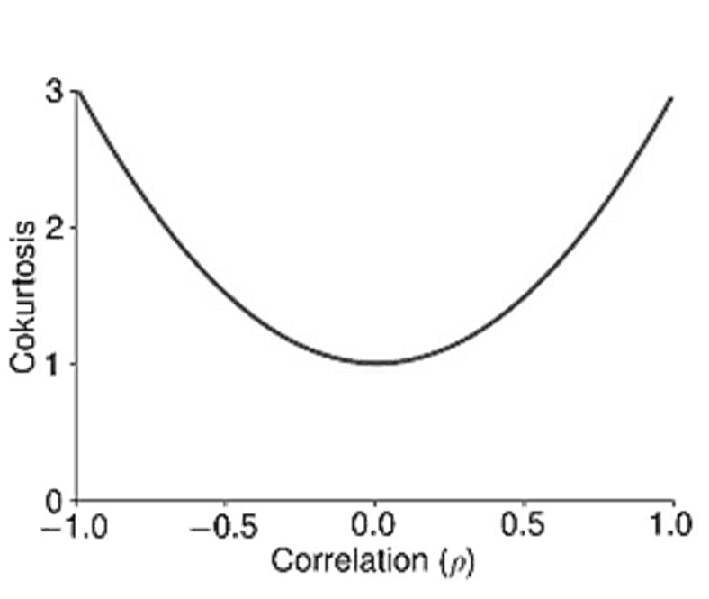
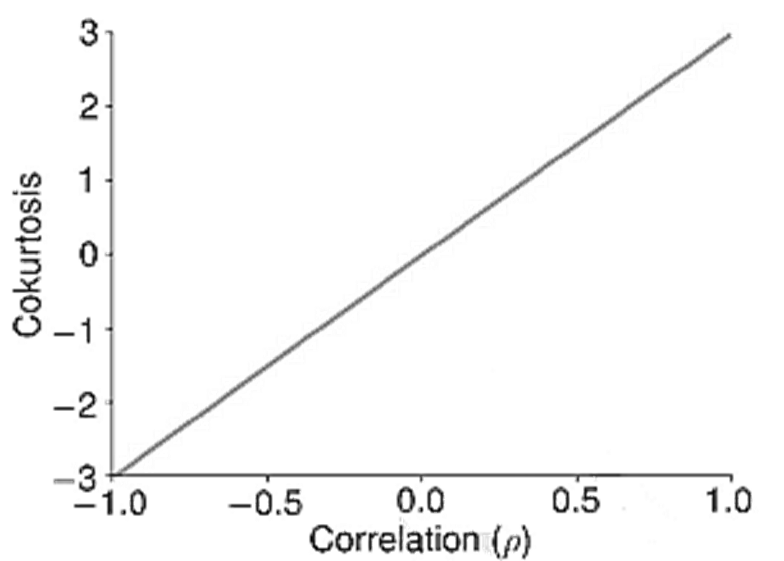
- The cokurtosis uses combinations of powers that add to 4, and so there are three configurations: (1,3), (2,2), and (3,1). The (2,2) measure is the easiest to understand and captures the sensitivity of the magnitude of one series to the magnitude of the other series. If both series tend to be large in magnitude at the same time, then the (2,2) cokurtosis is large. The other two kurtosis measures, (3,1) and (1,3), capture the agreement of the return signs when the power 3 return is large.
- The three measures of cokurtosis are defined as:
| X | Y | s(X,X,X) | s(X,X,Y) | s(X,Y,Y) | s(Y,Y,Y) |
| Bonds | Crude | -0.179 | -0.008 | 0.040 | 0.104 |
| Bonds | Gold | -0.179 | -0.018 | -0.032 | -0.101 |
| Bonds | Stocks | -0.179 | -0.082 | 0.012 | -0.365 |
| Crude | Gold | 0.104 | -0.010 | -0.098 | -0.101 |
| Crude | Stocks | 0.104 | -0.064 | -0.127 | -0.365 |
| Gold | Stocks | -0.101 | -0.005 | 0.014 | -0.365 |
| X | Y | k(X,X,X,X) | k(X,X,X,Y) | k(X,X,Y,Y) | k(X,Y,Y,Y) | k(X,Y,Y,Y) |
| Bonds | Crude | 6.662 | -0.248 | 1.996 | 0.244 | 15.656 |
| Bonds | Gold | 6.662 | -0.537 | 1.808 | 0.547 | 9.390 |
| Bonds | Stocks | 6.662 | -1.522 | 2.921 | 0.682 | 11.020 |
| Crude | Gold | 15.656 | 4.010 | 2.833 | 7.011 | 9.390 |
| Crude | Stocks | 15.656 | -0.443 | 2.490 | 4.750 | 11.020 |
| Gold | Stocks | 9.390 | -0.081 | 3.230 | 2.491 | 11.020 |
Standard Errors Versus Standard Deviation
- The variance of the sample mean depends on the variance of the data. The standard deviation of the mean estimator is
- The standard deviation of the mean (or any other estimator) is known as a standard error. Standard errors and standard deviations are similar, although these terms are not used interchangeably.
- Standard deviation refers to the uncertainty in a random variable or data set. Standard deviation does not change with the sample size.
- Standard error is used to refer to the uncertainty of an estimator. The standard error of an estimator declines as the sample size increases.
Presenting The Mean and Standard Deviation
- Means and standard deviations are the most widely reported statistics. Their popularity is due to several factors.
- The mean and standard deviation are often enough to describe the data.
- These two statistics provide guidance about the likely range of values that can be observed.
- The mean and standard deviation are in the same units as the data, and so can be easily compared.
- One challenge when using asset price data is the choice of sampling frequency. Most assets are priced at least once per day, and many assets have prices that are continuously available throughout the trading day (e.g., equities, some sovereign bonds, and futures). Other return series, such as hedge fund returns, are only available at lower frequencies (e.g., once per month). This can create challenges when describing the mean or standard deviation of financial returns.
- In practice, it is preferred to report the annualized mean and standard deviation, regardless of the sampling frequency. Annualized sample means are scaled by a constant that measures the number of sample periods in a year. For example, a monthly mean is multiplied by 12 to produce an annualized mean. Similarly, a weekly mean is multiplied by 52 to produce an annualized version, and a daily mean is multiplied by the number of trading days per year (e.g., 252 or 260). The scaling convention for daily statistics varies by country (and possibly by the year) because the number of trading days differs across markets..
- Meanwhile, standard deviations use the square root of the same scale factors. For example, the standard deviation computed from daily data is multiplied by √252 to produce an annualized standard deviation
Scaling of the Mean and Standard deviation
- Returns can also be measured using the difference between log prices (i.e., the natural logarithm of the returns).
- Log returns are convenient, as the two-period return is just the sum of two consecutive returns:
- If returns are iid with
- mean E[Ri]=μ, then the mean of the n-period return is nμ, because the expectation of the sum is the sum of the expectation.
- variance V[Ri]=σ^2 , and then the variance of the n-period return is nσ2, because the covariance between the returns is 0 due to the iid property
- In practice, financial returns are not iid but can be uncorrelated, which is sufficient for this relationship to hold.
- Standard deviation is the square root of the variance, and so the 𝑛-period standard deviation scales with √n.
Estimating the Mean and Variance using Data
- Consider a set of four data series extracted from the Federal Reserve Economic Data (FRED) database of the Federal Reserve Bank of St. Louis:
- The ICE BoAML US Corp Master Total Return Index Value, which measures the return on a diversified portfolio of corporate bonds;
- The Russell 2000 Index, a small-cap equity index that measures the average performance of 2,000 firms;
- The Gold Fixing Price in the London bullion market, the benchmark price for gold; and
- The spot price of West Texas Intermediate Crude Oil, the leading price series for US crude oil.
- All data in this set are from the period between January 1, 1987, and December 31, 2018. These prices are sampled daily, weekly (on Thursdays), and at the end of the month. Returns are computed using log returns, defined as the difference between consecutive log prices i.e.,
Higher Moments
| Daily Data | ||||
| Bonds | Stocks | Gold | Crude | |
| Mean | 0.027% | 0.044% | 0.020% | 0.044% |
| Std. Dev. | 0.301% | 1.295% | 1.002% | 2.496% |
| Skewness | -0.321 | -0.204 | -0.095 | 0.090 |
| Kurtosis | 5.62 | 9.41 | 9.56 | 15.75 |
| Ann. Mean | 6.9% | 11.2% | 5.2% | 11.1% |
| Ann. Std. Dev | 4.8% | 20.6% | 15.9% | 39.6 |
| n | 7,346 | 7,346 | 7,346 | 7,346 |
| n/Year | 245 | 245 | 245 | 245 |
| Weekly Data | ||||
| Bonds | Stocks | Gold | Crude | |
| Mean | 0.129% | 0.206% | 0.096% | 0.193% |
| Std. Dev. | 0.652% | 2.744% | 2.154% | 5.120% |
| Skewness | -0.397 | -0.678 | 0.211 | -0.076 |
| Kurtosis | 5.57 | 11.65 | 7.82 | 5.79 |
| Ann. Mean | 6.7% | 10.7% | 5.0% | 10.0% |
| Ann. Std. Dev | 4.7% | 19.86% | 15.5% | 36.9 |
| n | 1,565 | 1,565 | 1,565 | 1,565 |
| Monthly Data | ||||
| Bonds | Stocks | Gold | Crude | |
| Mean | 0.559% | 0.866% | 0.427% | 0.709% |
| Std. Dev. | 1.462% | 5.287% | 4.460% | 9.375% |
| Skewness | -0.745 | -0.443 | 0.146 | 0.275 |
| Kurtosis | 7.65 | 3.89 | 4.31 | 5.19 |
| Ann. Mean | 6.7% | 10.4% | 5.1% | 8.5% |
| Ann. Std. Dev | 5.1% | 18.3% | 15.4% | 32.5% |
| n | 359 | 359 | 359 | 359 |
- Skewness, while being unit-free, does not follow a simple scaling law across sampling frequencies.
- Financial data is heteroskedastic (i.e., the volatility of return changes over time) and the differences in the volatility dynamics across assets produce a different scaling of skewness.
- Gold has a positive skewness, especially at longer horizons, indicating that positive surprises are more likely than negative surprises.
- The skewness of crude oil returns is negative when returns are sampled at the daily horizon but becomes positive when sampling over longer horizons.
- Bond and stock market returns are usually negatively skewed.
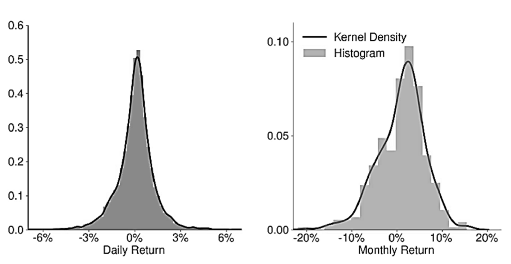
- All four asset returns series have excess kurtosis, although bonds have fewer extreme observations than the other three asset classes. Kurtosis declines at longer horizons, and it is a stylized fact that returns sampled at low frequencies (i.e., monthly, or even quarterly) have a distribution that is closer to that of a normal than returns sampled at higher frequencies. This is because large short-term changes are diluted over longer horizons by periods of relative calmness.
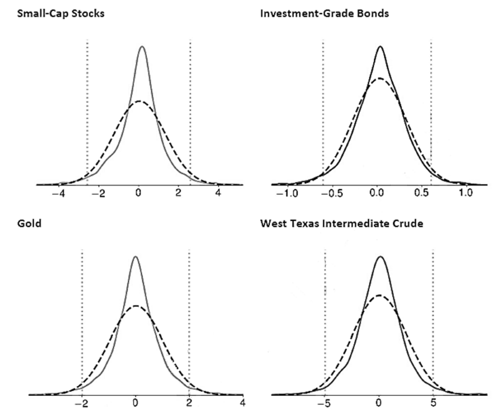
Histograms and Kneel Destiny Plots
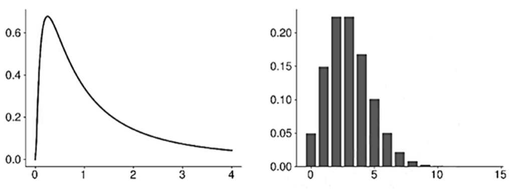
- Histograms are used to represent the frequency distribution of a data series. Histograms divide the range of the data into m bins and then tabulate the number of values that fall within the bounds of each bin.
- Kernel density plots are smoothed versions of histogram plots. Kernel density plots are generally preferred over histograms when visualizing the distribution of a dataset.
- A density plot differs from a histogram in two ways.
- First, rather than using discrete bins with well-defined edges, a density plot computes the number of observations that are close to any point on the x-axis. In effect, a density plot uses as many bins as there are data points in the sample.
- Second, a density plot uses a weighted count where the weight depends on the distance between the point on the x-axis and the observed value. Most common kernel density estimators use a weight function that declines as the distance between two points increases, thus producing a smooth curve.
The Blue Mean Estimator
- The mean estimator is the Best Linear Unbiased Estimator (BLUE) of the population mean when the data are iid. In this context, best indicates that the mean estimator has the lowest variance of any linear unbiased estimator (LUE).
- Linear estimators of the mean can be expressed as:
- BLUE is a desirable property for an estimator, because it establishes that the estimator is the best estimator (in the sense of having the smallest variance) among all linear and unbiased estimators.
- There can be superior estimators to the sample mean, but these estimators are either biased or nonlinear. Maximum likelihood estimators of the mean are generally more accurate than the sample mean, although they are usually nonlinear and often biased in finite samples.
Large Sample Behavior of the Mean
- If data are iid normally distributed, then the mean estimator is also normally distributed, if the sample size is large enough.
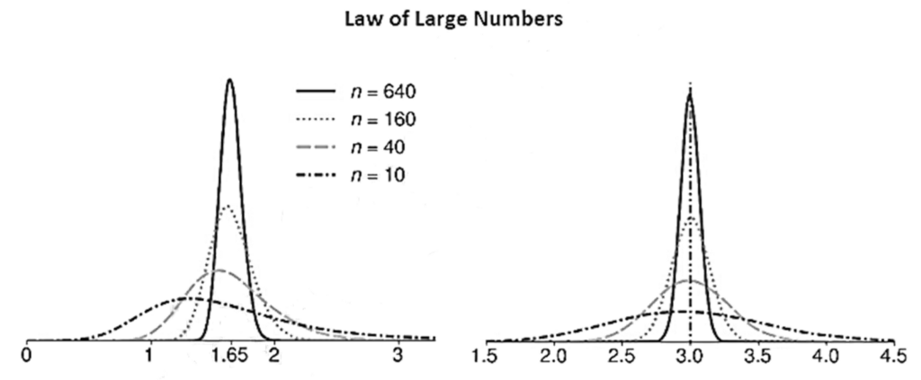
- The Law of Large Numbers (LLN) establishes the large sample behavior of the mean estimator and provides conditions where an average converges to its expectation.
- The simplest LLN for iid random variables is the Kolmogorov Strong Law of Large Numbers. This LLN states that if {X_i} is a sequence of iid random variables with μ≡E[X_i], then:
- When an LLN applies to an estimator, the estimator is said to be consistent.
- Consistency requires that an estimator is asymptotically unbiased, and so any finite sample bias must diminish as 𝑛 increases (e.g., σ ̂2 has this property).
- A consistent estimator has another key feature: as the sample size 𝑛 grows larger, the variance of the estimator converges to zero (i.e., V[μ ̂n]→0). This ensures that the chance of observing a large deviation from the population value is negligible in large samples.
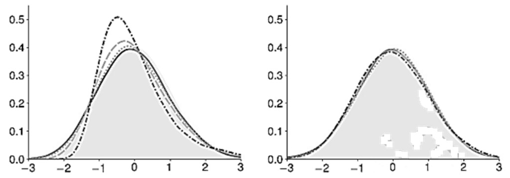
- Two features are evident from the LLN plots. .
- First, the density of the sample mean is not a normal. In sample means computed from the simulated log-normal data, the distribution of the sample mean is right-skewed, especially when n is small.
- Second, the distribution becomes narrower and more concentrated around the population mean as the sample size increases. The collapse of the distribution around the population mean is evidence that the LLN applies to these estimators.
- The LLN also applies to other sample moments. For example, when the data are iid and E[Xi^2] is finite, then the LLN ensures that σ ̂2 →┴(a.s.) σ2, and so the sample variance estimator is also consistent.
- Consistency is an important property of an estimator, although it is not enough to understand its distribution. For example, distribution of μ ̂-μ is not easy to study because it collapses to 0 as n→∞.
- The solution is to rescale the difference between the estimate and population value by √𝑛. This is the precise value that stabilizes the distribution because
Central Limit Theorem
- The CLT can also be applied to the rescaled difference under some additional assumptions.
- The simplest CLT is known as the Lindberg-Lévy CLT. This CLT requires one additional assumption that the variance σ^2 is finite. It states that if {Xi} are iid, then
- This CLT can be alternatively expressed as:
Large Sample Behavior of the Mean
- CLTs extend LLNs and provide an approximation to the distribution of the sample mean estimator. Furthermore, they do not require knowledge of the distribution of the random variables generating the data. In fact, only independence and some moment conditions are required for the CLT to apply to a sample mean estimator.
- In practice, the CLT is used as an approximation in finite samples so that the distribution of the sample mean is approximated by:
The Median and Other Quantiles
- The median, like the mean, measures the central tendency of a distribution. Specifically, it is the 50% quantile of the distribution and the point where the probabilities of observing a value above or below it are equal (i.e., 50%).
- When a distribution is symmetric, the median is in the center of the distribution and is the same as the mean.
- When distributions are asymmetric, the median is larger (smaller) than the mean if the distribution is left-skewed (right-skewed).
- Estimation of the median is simple. First, the data are sorted from smallest to largest.
- When the sample size is odd, the value in position (n + 1)/2 of the sorted list is used to estimate the median:
- When the sample size is even, the median is estimated using the average of the two central points of the sorted list:
- Two other commonly reported quantiles are the 25% and 75% quantiles. These are estimated using the same method as the median.
- More generally, the α-quantile is estimated from the sorted data using the value in location 𝛼𝑛. When 𝛼𝑛 is not an integer value, then the usual practice is to take the average of the points immediately above and below αn.
- These two quantile estimates (q ̂_25and q ̂_75) are frequently used together to estimate the interquartile range:
- The IQR is a measure of dispersion and so is an alternative to standard deviation. Other quantile measures can be constructed to measure the extent to which the series is asymmetric or to estimate the heaviness of the tails.
- Two features make quantiles attractive.
- First, quantiles have the same units as the underlying data, and so they are easy to interpret. For example, the 25% quantile for a sample of asset returns estimates the point where there is 25% probability of observing a smaller return (and a 75% probability of observing a larger return). Meanwhile, the interquartile range estimates a central interval where there is 50% probability of observing a return.
- Second, quantiles are robustness to outliers. For example, suppose that some observed data {x1, … , xn} are contaminated with an outlier. Both the median and IQR are unaffected by the presence of an outlier. However, this is not true of the mean estimator, which gives weight 1/n to the outlier. If the outlier is far from the other (valid) observations, this distortion can be large. The variance, because it squares the difference between the outlier and the mean, is even more sensitive to outliers.
| Daily Data | ||||
| Bonds | Stocks | Gold | Crude | |
| Median | 0.034% | 0.103% | 0.014% | 0.058% |
| q(.25) | -0.140% | -0.534% | -0.445% | -1.21% |
| q(.75) | 0.207% | 0.660% | 0.496% | 1.30% |
| IQR | 0.347% | 1.19% | 0.941% | 2.51% |
| Weekly Data | ||||
| Bonds | Stocks | Gold | Crude | |
| Median | 0.159% | 0.459% | 0.044% | 0.224% |
| q(.25) | -0.244% | -1.12% | -1.01% | -2.64% |
| q(.75) | 0.542% | 1.69% | 1.24% | 3.03% |
| IQR | 0.786% | 2.81% | 2.24% | 5.67% |
| Monthly Data | ||||
| Bonds | Stocks | Gold | Crude | |
| Median | 0.640% | 1.56% | 0.265% | 0.839% |
| q(.25) | -0.220% | -2.47% | -2.29% | -5.14% |
| q(.75) | 1.42% | 4.12% | 2.84% | 6.72% |
| IQR | 1.64% | 6.59% | 5.14% | 11.9% |
Covariance and Correlation
- Covariance measures the linear dependence between two random variables and is defined as:
- The sample covariance estimator uses the sample analog to the expectation operator
Multivariate Moments
- Correlation is the standardized version of the covariance and is usually preferred because it does not depend on the scale of X or Y. The correlation is estimated by dividing the sample covariance by the product of the sample standard deviations of each asset:
- The sample correlation estimator is biased in finite samples, even if unbiased estimators are used to estimate the variances and covariance.
| Daily Data | ||||
| Bonds | Stocks | Gold | Crude | |
| Bonds | — | -16.4% | 3.0% | -9.9% |
| Stocks | -16.4% | — | -2.1% | 12.5% |
| Gold | 3.0% | -2.1% | — | 13.0% |
| Crude | -9.9% | 12.5% | 13.0% | — |
| Weekly Data | ||||
| Bonds | Stocks | Gold | Crude | |
| Bonds | — | -2.4% | 2.3% | -7.7% |
| Stocks | -2.4% | — | 4.0% | 13.2% |
| Gold | 2.3% | 4.0% | — | 15.2% |
| Crude | -7.7% | 13.2% | 15.2% | — |
| Monthly Data | ||||
| Bonds | Stocks | Gold | Crude | |
| Bonds | — | 15.1% | 19.6% | -0.2% |
| Stocks | 15.1% | — | -0.2% | 11.6% |
| Gold | 19.6% | -0.2% | — | 18.9% |
| Crude | -0.2% | 11.6% | 18.9% | — |
Sample Mean of Two Variables
- Estimating the means of two random variables is no different from estimating the mean of each separately, so that:
- When data are iid, the CLT applies to each estimator. However, it is more useful to consider the joint behavior of the two mean estimators by treating them as a bivariate statistic. The CLT can be applied by stacking the two mean estimators into a vector:
Multivariate Moments
- The CLT for the vector depends on the 2-by-2 covariance matrix for the data. The CLT for a pair of mean estimators is virtually identical to that of a single mean estimator, where the scalar variance is replaced by the covariance matrix. The CLT for bivariate iid data series states that:
- In practice, this CLT is applied by treating the mean estimators as a bivariate normal random variable:
- Applying the bivariate CLT:
- The most important insight from the bivariate CLT is that correlation in the data produces a correlation between the sample means. Moreover, the correlation between the means is identical to the correlation between the data series.
| Moment | μ̂_X | σ_S^2 | μ̂_X | σ_B^2 | σ_SB | ρ |
| 10.4 | 335.4 | 6.71 | 25.6 | 14.0 | 0.151 |
Coskewness and Cokurtosis
- Like variance, skewness and kurtosis can be extended to pairs of random variables. When computing cross pth moments, there are p-1 different measures. Applying the principle to the first four moments there are
- No cross means,
- One cross variance (covariance),
- Two measures of cross-skewness (coskewness), and
- Three cross-kurtoses (cokurtosis).
- The two coskewness measures are
- The coskewness standardizes the cross-third moments by the variance of one of the variables and the standard deviation of the other, and so is scale- and unit-free.
- These measures both capture the likelihood of the data taking a large directional value whenever the other variable is large in magnitude. When there is no sensitivity to the direction of one variable to the magnitude of the other, the two coskewnesses are 0. For example, the coskewness in a bivariate normal is always 0, even when the correlation is different from 0.
- The univariate skewness estimators are s(X, X, X) and s(Y, Y, Y).
Multivariate Moments
- Coskewnesses are estimated by applying the sample analog to the expectation operator to the definition of coskewness. For example:
- The cokurtosis uses combinations of powers that add to 4, and so there are three configurations: (1,3), (2,2), and (3,1). The (2,2) measure is the easiest to understand and captures the sensitivity of the magnitude of one series to the magnitude of the other series. If both series tend to be large in magnitude at the same time, then the (2,2) cokurtosis is large. The other two kurtosis measures, (3,1) and (1,3), capture the agreement of the return signs when the power 3 return is large.
- The three measures of cokurtosis are defined as:
| X | Y | s(X,X,X) | s(X,X,Y) | s(X,Y,Y) | s(Y,Y,Y) |
| Bonds | Crude | -0.179 | -0.008 | 0.040 | 0.104 |
| Bonds | Gold | -0.179 | -0.018 | -0.032 | -0.101 |
| Bonds | Stocks | -0.179 | -0.082 | 0.012 | -0.365 |
| Crude | Gold | 0.104 | -0.010 | -0.098 | -0.101 |
| Crude | Stocks | 0.104 | -0.064 | -0.127 | -0.365 |
| Gold | Stocks | -0.101 | -0.005 | 0.014 | -0.365 |
| X | Y | k(X,X,X,X) | k(X,X,X,Y) | k(X,X,Y,Y) | k(X,Y,Y,Y) | k(X,Y,Y,Y) |
| Bonds | Crude | 6.662 | -0.248 | 1.996 | 0.244 | 15.656 |
| Bonds | Gold | 6.662 | -0.537 | 1.808 | 0.547 | 9.390 |
| Bonds | Stocks | 6.662 | -1.522 | 2.921 | 0.682 | 11.020 |
| Crude | Gold | 15.656 | 4.010 | 2.833 | 7.011 | 9.390 |
| Crude | Stocks | 15.656 | -0.443 | 2.490 | 4.750 | 11.020 |
| Gold | Stocks | 9.390 | -0.081 | 3.230 | 2.491 | 11.020 |
Go to Syllabus
Courses Offered
Popular Courses
FRM Part 1
FRM Part 2

By : Micky Midha
9 Hrs of Videos
Available On Web, IOS & Android
Access Until You Pass
Lecture PDFs
Class Notes

By : Micky Midha
12 Hrs of Videos
Available On Web, IOS & Android
Access Until You Pass
Lecture PDFs
Class Notes

By : Micky Midha
257 Hrs Of Videos
Available On Web, IOS & Android
Access Until You Pass
Complete Study Material
Quizzes,Question Bank & Mock tests

By : Micky Midha
240 Hrs Of Videos
Available On Web, IOS & Android
Access Until You Pass
Complete Study Material
Quizzes,Question Bank & Mock tests

By : Shubham Swaraj
Lecture Videos
Available On Web, IOS & Android
Complete Study Material
Question Bank & Lecture PDFs
Doubt-Solving Forum