What is a multivariate random variable ?

A multivariate random variable is a vector of two or more random variables, each representing a univariate random variable.

What is a bivariate random variable ?

A bivariate random variable consists of two components, each representing a different random variable.

How is a probability mass function (PMF) used ?

A PMF for a bivariate random variable returns the probability that each random variable takes a specific value.

What is a marginal distribution ?

A marginal distribution is the distribution of a single component of a bivariate random variable.

Covariance measures how two random variables move together, indicating the direction of their relationship.

What is correlation ?

Correlation is a standardized measure of the strength and direction of a linear relationship between two variables.

What is conditional distribution ?

A conditional distribution gives the probability of outcomes for one random variable given a specific value of another.

How is covariance related to portfolio diversification ?

Covariance helps in understanding how different assets move together, affecting portfolio risk.

What is a conditional expectation ?

Conditional expectation is the expected value of a random variable given that another variable takes a specific value.

What are cross central moments ?

Cross central moments generalize covariance and include coskewness and cokurtosis, measuring extreme deviations.

Multivariate Random Variables

Introduction

Multivariate random variables extend the concept of a single random variable to include measures of dependence between two or more random variables. Each component of a multivariate random variable is a univariate random variable.
Multivariate random variables are vectors of random variables. For example, a bivariate random variable 𝑋 would be a vector with two components: and $X_2$ . Similarly, its realization (i.e., x) would have two component values as well: $x_1$ and $x_2$ . Treated separately, $x_1$ is a realization from from $X_1$ and $x_2$ is a realization from $X_2$ .
Just like their univariate counterparts, multivariate random variables are like in that they can be discrete or continuous. Similarly, both types of random variables are denoted with uppercase letters (e.g., X, Y, or Z).
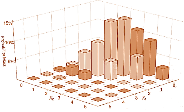
The probability mass function (PMF) for a bivariate random variable returns the probability that two random variables each take a certain value. This means that plotting these functions requires three axes: $X_1$ , $X_2$ , and the probability mass/density. The CDF requires three axes as well.

Bivariate Random Variable

The PMF of a bivariate random variable is given by

$f_{X_1,X_2}(x_1,x_2)=P(X_1=x_1,X_2=x_2)$

An example of a discrete bivariate random variable is the trinomial distribution, which is the distribution of n independent trials where each trial produces one of three outcomes.

The two components of a trinomial are $X_1$ and $X_2$ , which count the number of realizations of outcome 1 and 2. The count of the realizations for outcome 3 is given by $n-X_1-X_2$ .
For example, when measuring the credit quality of a diversified bond portfolio, the 𝑛 bonds can be classified as investment grade, high yield or unrated. In this case, $X_1$ is the count of the investment grade bonds and $X_2$ is the count of the high yield bonds.

The trinomial PMF has three parameters:

n (i.e., the total number of experiments),

$p_1$ , (i.e., the probability of observing outcome 1), and

$p_2$ (i.e., the probability of observing outcome 2).

Because these outcomes are exclusive, the probability of outcome 3 is simply

$p_3=1-p_2-p_1$

•The PMF of a trinomial random variable is

$f_{X_1,X_2}(x_1,x_2)=\frac{n!}{x_1!x_2!(n-x_1-x_2)!}p_1^{x_1}p_2^{x_2}(1-p_1-p_2)^{n-x_1-x_2}$

The CDF of a bivariate variable is a function returning the total probability that each component is less than or equal to a given value for that component, so that:

$F_{X_1,X_2}(x_1,x_2)=\sum_{t_1\in R(X_1)\atop t_1\leq x_1}\sum_{t_2\in R(X_2)\atop t_2\leq x_2}f_{X_1,X_2}(t_1,t_2)$

where $t_1$ contains the values that $X_1$ may take as long as $t_1\leq x_1$ , and

$t_1$ is similarly defined only for $X_2$ .

Joint Probabilities

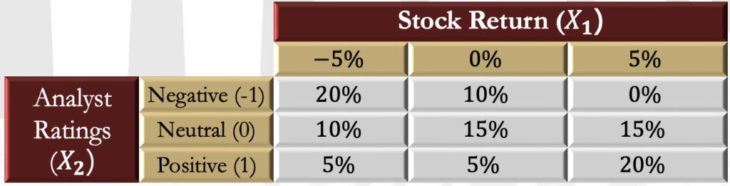
Discrete distributions defined over a finite set of values can be described using a probability matrix, which relates realizations to probabilities. In other words, it is a tabular representation of a PMF.
For example, let the return on a company’s stock be related to the rating given to the company by an analyst. Assume that the stock can only have three possible returns: 0, 5%, or -5%. Analyst ratings can be positive, neutral, or negative, and are labeled 1, 0, or -1 (respectively).

Discrete distributions defined over a finite set of values can be described using a probability matrix, which relates realizations to probabilities. In other words, it is a tabular representation of a PMF.
For example, let the return on a company’s stock be related to the rating given to the company by an analyst. Assume that the stock can only have three possible returns: 0, 5%, or -5%. Analyst ratings can be positive, neutral, or negative, and are labeled 1, 0, or -1 (respectively).

Marginal Distributions

The PMF describes the joint distribution of the two components $[\text{i.e.,}\Pr(X_1=x_1,X_2=x_2)]$ . It is also possible to examine each variable individually.

The distribution of a single component of a bivariate random variable is called a marginal distribution. This distribution contains the probabilities of realizations of $X_1$ and its PMF denoted by $f_{X_1}(x_1)$ . Marginal PMF is simply a univariate PMF.

The marginal PMF of $X_1$ can be computed by summing the probability for each realization of $X_1$ across all values in the support of $X_2$ . The marginal PMF is defined as:

$f_{X_1}(x_1)=\sum_{x_2\in R(X_2)}f_{X_1,X_2}(x_1,x_2)$

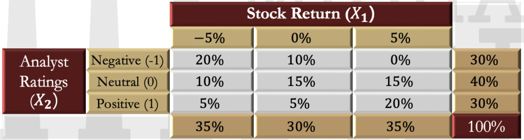
When a PMF is represented as a probability matrix, the two marginal distributions are computed by summing across columns (which constructs the marginal distribution of the row variables) or summing down rows (which constructs the marginal PMF for the column variables).

		Stock Return (X₁)			f_X2(X₂)
		−5%	0%	5%	f_X2(X₂)
Analyst Ratings (X₂)	Negative (-1)	20%	10%	0%	30%
	Neutral (0)	10%	15%	15%	40%
	Positive (1)	5%	5%	20%	30%
		35%	30%	35%	100%

•The marginal CDF is defined in a natural way using the marginal PMF so that $P(X_1<x_1)$ measures the total probability in the marginal PMF less than $x_1$

$F_{X_1}(x_1)=\sum_{t_1\leq x_1}\sum_{t_2\in R(X_1)}f_{X_1}(t_1)$

Independence

The components of a bivariate random variable are independent if

$f_{X_1,X_2}(x_1,x_2)=f_{X_1}(x_1)f_{X_2}(x_2)$

Independence requires that the joint PMF of $X_1\;and\;X_2$ be the product of the marginal PMFs.

Conditional Distributions

The conditional distribution, on the other hand, summarizes the probability of the outcomes for one random variable conditional on the other taking a specific value. The conditional probability of two events was defined as:

$P(A\mid B)=\frac{P(A\cap B)}{P(B)}$

This definition of conditional probability can be applied to a bivariate random variable to construct a conditional distribution. The conditional distribution of $X_1$ given $X_2$ is defined as:

$f_{X_1\mid X_2}(x_1\mid X_2=x_2)=\frac{f_{X_1,X_2}(x_1,x_2)}{f_{X_2}(x_2)}$

In other words, it is the joint probability of the two events divided by the marginal probability that $X_2=x_2$ .

For example, the distribution of stock returns conditional on a positive analyst rating is

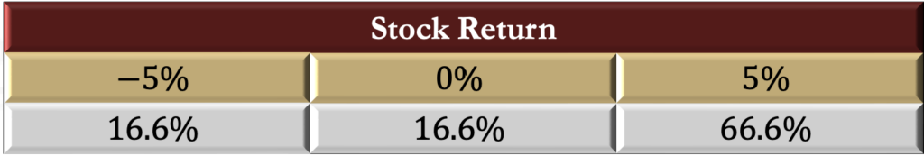
$f_{X_1\mid X_2}(x_1\mid X_2=1)=\frac{f_{X_1,X_2}(x_1,1)}{f_{X_2}(1)}=\frac{f_{X_1,X_2}(x_1,1)}{0.3}$

Conditional distributions can also be defined over a set of outcomes for one of the variables. For example, consider the distribution of the stock return given that the analyst did not give a positive rating. This set is

$X_2\in\{-1,0\}$

The conditional PMF must sum across all outcomes in the set that is conditioned on S={-1,0}, and so:

$f_{X_1|X_2}(x_1|X_2\in\{-1,0\})=\frac{\sum\limits_{x_2\in\{-1,0\}}f_{X_1,X_2}(x_1,x_2)}{\sum\limits_{x_2\in\{-1,0\}}f_{X_2}(x_2)}$

The marginal probability that $X_2\in\{-1,0\}$ is the sum of the (marginal) probabilities of these two outcomes:

$f_{X_2}(-1)+f_{X_2}(0)=70\%$

The conditional probability distribution is then:

$f_{X_1|X_2}(x_1|X_2\in\{-1,0\})=\left\{\begin{array}{c}\frac{\text{20\%}+\text{10\%}}{\text{70\%}}\quad=\quad\text{42.8\%}\\[10pt]\frac{\text{10\%}+\text{15\%}}{\text{70\%}}\quad=\quad\text{35.7\%}\\[10pt]\frac{\text{0\%}+\text{15\%}}{\text{70\%}}\quad=\quad\text{21.4\%}\end{array}\right.$

Independence

The definition of a conditional distribution can also be rearranged so that the joint PMF is expressed in terms of the marginal PMF and a conditional PMF. For example:

$\begin{aligned}f_{X_1,X_2}(x_1,x_2)&=f_{X_1|X_2}(x_1|X_2=x_2)f_{X_2}(x_2)\\&\text{or}\\f_{X_1,X_2}(x_1,x_2)&=f_{X_2|X_1}(x_2|X_1=x_1)f_{X_1}(x_1)\end{aligned}$

Equality of the conditional and the marginal PMFs is a requirement of independence. Specifically, knowledge about the value of $X_2$ (e.g., $X_2=x_2$ ) must not contain any information about $X_1$ .

Expectations

The expectation of a function of a bivariate random variable is defined analogously to that of a univariate random variable. The expectation of a function $g(X_1,X_2)$ is a probability weighted average of the function of the outcomes $g(x_1,x_2)$ . The expectation is defined as:

$\begin{equation}E[g(X_1,X_2)]=\sum_{x_1\in R(X_1)}\sum_{x_2\in R(X_2)}g(x_1,x_2)f_{X_1,X_2}(x_1,x_2)\end{equation}$

While $g(x_1,x_2)$ depends on $x_1\;and\;x_2$ , it may be a function of only one of the components.

As in the univariate case, $E[g(X_1,X_2)]\neq g(E[X_1],E[X_2])$ for a nonlinear function $g(x_1,x_2)$ .

As an example, consider the following joint PMF:

Now, consider the function

$g(x_1,x_2)=x_1^{x_2}$

The expectation of $g(x_1,x_2)$ is therefore

$E[g(X_1,X_2)]=\sum_{x_1\in\{1,2\}}\sum_{x_2\in\{3,4\}}g(x_1,x_2)f(x_1,x_2)$

Moments

The first moment of X (i.e., the mean E[X]) is the mean of the components

$E[X]=\left[E[X_1]E[X_2]\right]=\left[\mu_1,\mu_2\right]$

The second moment of X is referred to as the covariance of X. The covariance is technically a 2-by-2 matrix of values, where the values along one diagonal are the variances of $X_1\;and\;X_2$ , and the terms in the other diagonal are the covariance between $X_1\;and\;X_2$

The covariance is a measure of dispersion that captures how the variables move together.

The covariance between $X_1\;and\;X_2$ is defined as:

$\text{Cov}[X_1,X_2]=E[(X_1-E[X_1])(X_2-E[X_2])]=E[X_1 X_2]-E[X_1]E[X_2]$

Note that it is a generalization of the variance, and the covariance of a variable with itself is just the variance of that variable

Variances And Covariance

In a bivariate random variable, there are two variances and one covariance.

It is common to express $V[X_1]$ as $\sigma_{1}^{2}$ and $V[X_2]$ as $\sigma_{2}^{2}$ . The symbols $\sigma_1\;and\;\sigma_2$ are used to denote the standard deviations of $X_1\;and\;X_2$ , respectively.

An alternative abbreviation scheme uses $\sigma_{11}\;and\;\sigma_{22}$ to indicate the variances of $X_1\;and\;X_2$ , respectively.
The covariance is commonly abbreviated to $\sigma_{12}$ in both schemes.

Covariance And Correlation

Covariance is difficult to interpret because it can take on values from -∞ to +∞. It can be made easier to interpret by standardizing it to produce correlation. It is therefore more common to report the correlation, which is a scale-free measure. Correlation of two variables is obtained by dividing their covariance by their respective standard deviations i.e.

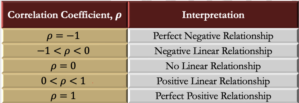
$\text{Corr}[X_1,X_2]=\frac{\text{Cov}[X_1,X_2]}{\sqrt{V[X_1]V[X_2]}}=\frac{\sigma_{12}}{\sqrt{\sigma_1^2\sigma_2^2}}=\frac{\sigma_{12}}{\sigma_1\sigma_2}$

Correlation measures the strength of the linear relationship between two variables and is always between -1 and 1. When $X_1\;and\;X_2$ tend to increase together, then the correlation is positive. If $X_2$ tends to decrease when $X_1$ increases, then these two random variables have a negative correlation.

Shifting And Scaling Effects On Covariance

Location shifts have no effect on the covariance, whereas the scale of each component contributes multiplicatively to the change in the covariance. Hence,

Applying location shifts of a and c

AND

rescaling the variables by b and d scales the covariance by bd. i.e.

$\text{Cov}[a+bX_1,c+dX_2]=bd\,\text{Cov}[X_1,X_2]$

Using the above, the correlation estimator is scale free:

$\text{Corr}[aX_1,bX_2]=\frac{ab\,\text{Cov}[X_1,X_2]}{\sqrt{a^2V[X_1]}\sqrt{b^2V[X_2]}}=\frac{ab}{|a||b|}\frac{\text{Cov}[X_1,X_2]}{\sqrt{V[X_1]}\sqrt{V[X_2]}}=\text{sign}(a)\text{sign}(b)\text{Corr}[X_1,X_2]$

Covariance – Properties

$Cov(X_1,X_2)=0$ where $X_1\;and\;X_2$ are independent random variables.

$Cov(X_1,X_1)=Var(X_1)$ i.e. the covariance of a random variableX_1with itself is the variance of X_1.

$\text{Cov}[a+bX_1,c+dX_2]=bd\times\text{Cov}[X_1,X_2]$ where a, b, c, d are constants.

$V[X_1+X_2]=V[X_1]+V[X_2]+2\times\text{Cov}[X_1,X_2]$

$V[X_1-X_2]=V[X_1]+V[X_2]-2\times\text{Cov}[X_1,X_2]$

if $X_1\;and\;X_2$ are not independent $V[aX_1+bX_2]=a^2 V[X_1]+b^2 V[X_2]+2ab\times\text{Cov}[X_1,X_2]$

Covariance Matrix

The correlation between two random variables is commonly denoted by ρ (or $\rho_{12}$ to specify that this is the correlation between the components). The covariance can be expressed in terms of the correlation and the standard deviations:

$\sigma_{12}=\rho_{12}\sigma_1\sigma_2$

The variance of each component and the covariance between the two components of X are frequently expressed as a 2-by-2 covariance matrix. The covariance matrix of X is

$\text{Cov}[X]=\begin{bmatrix}\sigma_1^2&\sigma_{12}\\\sigma_{12}&\sigma_2^2\end{bmatrix}=\begin{bmatrix}\sigma_{11}&\sigma_{12}\\\sigma_{12}&\sigma_{22}\end{bmatrix}$

Correlation Interpretation

The following table shows the interpretation of different values of correlation

Correlation And Portfolio Diversification

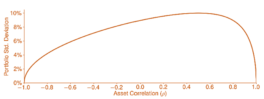
The portfolio standard deviation using the optimal portfolio weight in a two-asset portfolio, where the first asset has a volatility of 20%, the second has a volatility of 10%, and the correlation between the two is varied between -1 and 1.

Covariance, Correlation, And Independence

When two random variables are independent, they must have zero correlation because (by definition) they must contain no information about each other. However, if two random variables have zero correlation, they are not necessarily independent.

Correlation is a measure of linear dependence. If two variables have a strong linear relationship (i.e., they produce values that lie close to a straight line), then they have a large correlation. If two random variables have no linear relationship, then their correlation is zero.

However, variables can be non-linearly dependent. A simple example of this occurs when:

$X_1\sim N(0,1)\;\text{and}\;X_2=X_1^2$

It is known that

$Cov[X_1 X_2]=E[X_1 X_2]-E[X_1]E[X_2]$

If the correlation between two variables is 0, then $Cov[X_1 X_2]=0$ , so

$E[X_1 X_2]=E[X_1]E[X_2]$

Hence, the expectation of the product of the two is the product of the expectations when the two variables are linearly independent.

Cross Central Moments

The concept of covariance can be generalized and cross central moments can be identified.
The third cross central moment is known as coskewness. If two random variables exhibit positive coskewness they will tend to undergo extreme positive deviations at the same time. Similarly, if two random variables exhibit negative coskewness they will tend to undergo extreme negative deviations at the same time.
The fourth cross central moment is known as cokurtosis. If two random variables exhibit a high level of cokurtosis they will tend to undergo extreme positive and negative deviations at the same time.

Coskewness and Cokurtosis are defined by taking powers of the two variables that sum to 3 or 4, respectively. There are two distinct coskewness measures and three distinct cokurtosis measures.

For example, the two coskewness measures are

$\frac{E\left[(X_1-E[X_1])^2(X_2-E[X_2])\right]}{\sigma_1^2\sigma_2}\quad\text{and}\quad\frac{E\left[(X_1-E[X_1])(X_2-E[X_2])^2\right]}{\sigma_1\sigma_2^2}$

Like the skewness of a single random variable, the coskewness measures are standardized.

They both measure whether one random variable (raised to the power 1) takes a clear direction whenever the other return (raised to the power 2) is large in magnitude. For example, it is common for returns on individual stocks to have negative coskew, so that when one return is negative, the other tends to experience a period of high volatility (i.e., its squared value is large).

Conditional Expectations

A conditional expectation is an expectation when one random variable takes a specific value or falls into a defined range of values. It uses the same expression as any other expectation and is a weighted average where the probabilities are determined by a conditional PMF.

In the previous example, consider the expected return on the stock given a positive analyst rating. The conditional distribution here [i.e., $f_{X_1|X_2}(x_1|X_2=1)$ ] is

The conditional expectation of the return is

$E[X_1|X_2=1]=$

Conditional Moments

Conditional expectations can be extended to any moment by replacing all expectation operators with conditional expectation operators. For example, the variance of a random variable X_1 is

$V[X_1]=E[(X_1-E[X_1])^2]=E[X_1^2]-E[X_1]^2$

The conditional variance of $X_1$ given $X_2$ is

$V[X_1|X_2=x_2]=E[(X_1-E[X_1|X_2=x_2])^2|X_2=x_2]=E[X_1^2|X_2=x_2]-E[X_1|X_2=x_2]^2$

In the previous example, the standard deviation of the stock return (i.e., the square root of the variance) is

$\sigma_1=\sqrt{V(X_1)}=\sqrt{E[X_1^2]-E[X_1]^2}$

The standard deviation conditional on a positive rating is

$\sigma_{x_1|x_2=1}=\sqrt{V(X_1|X_2=1)}=\sqrt{E[X_1^2|X_2=1]-E[X_1|X_2=1]^2}$

Conditional Independence

As a rule, random variables are dependent in finance and risk management. This dependence arises from many sources, including
- shifts in investor risk aversion,
- cross-asset or cross-border spillovers, and
- crowded portfolio strategies.
Conditioning is a useful tool to remove the dependence between variables.

In the previous example, suppose that an investor wants to identify firms that have a conservative management style. This style variable can be labeled Z.
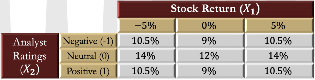
Now suppose that 12.5% of the companies are in the conservative category and that the probability of the outcomes of stock returns and recommendations based on management style are as in the table below:

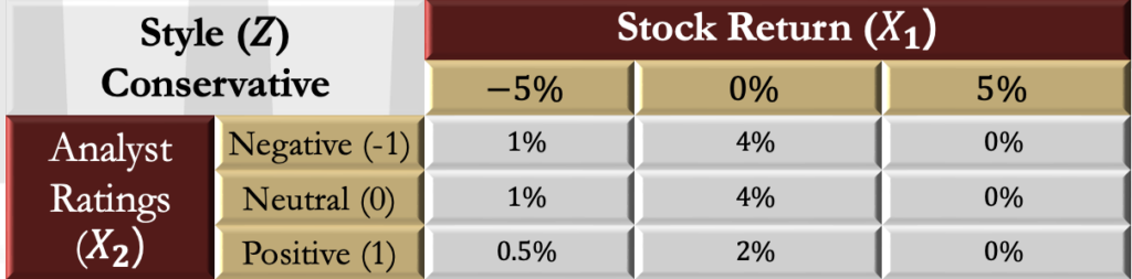
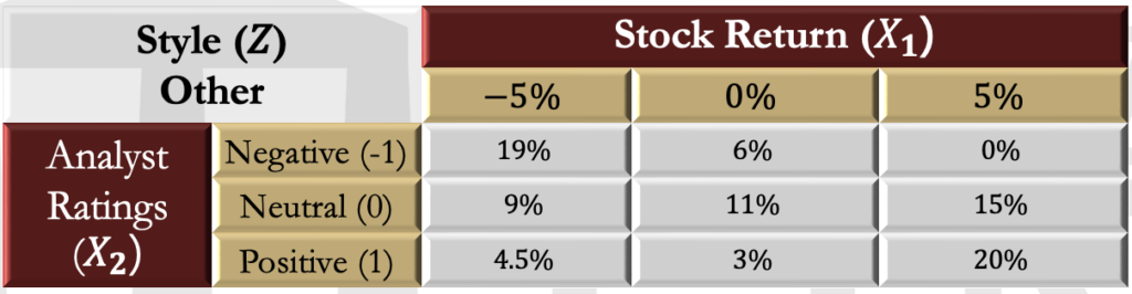
The overall probabilities are consistent with the original bivariate matrix. For example, there is still a total 20% chance of a negative rating when the stock return is -5%.

Now consider the bivariate distribution conditional on a company being in this conservative category. As before, each individual probability is rescaled by a constant factor so that the total conditional probability sums to 1. In other words, each value is divided by the probability that the management is conservative (i.e., 12.5%), which is also the sum of the values in the panel.

Continuous Random Variables

Moving from discrete multivariate random variables to those that are continuous changes little. The most substantial change is the replacement of the PMF with a PDF, and the corresponding switch from sums to integrals when computing expectations. All definitions and high-level results (e.g., the effect of linear transformations on the covariance of random variables) are identical.

The PDF has the same form as a PMF and is written as

$f_{X_1,X_2}(x_1,x_2)$

The probability in a rectangular region is defined as:

$\text{Pr}(l_1<X_1<u_1\cap l_2<X_2<u_2)=\int_{l_1}^{u_1}\int_{l_2}^{u_2}f_{X_1,X_2}(x_1,x_2)\,dx_1\,dx_2$

This expression computes the volume under the PDF function in the region defined by $l_1$ , $u_1$ , $l_2$ , and $u_2$ . A PDF function is always non-negative and must integrate to one across the support of the two components.

The cumulative distribution function is the area of a rectangular region under the PDF where the lower bounds are -∞ and the upper bounds are the arguments in the CDF:

$F_{X_1,X_2}(x_1,x_2)=\int_{-\infty}^{x_1}\int_{-\infty}^{x_2}f(t_1,t_2)\,dt_1\,dt_2$

If the PDF is not defined for all values, then the lower bounds can be adjusted to be the smallest values where the random variable has support.

Most continuous multivariate random variables have complicated PDFs. The simplest is the standard bivariate uniform where the two components are independent. The PDF of this random variable is constant:

$f_{X_1,X_2}(x_1,x_2)=k$

and the support of the density is the unit square (i.e., a square whose sides have lengths of 1).

The CDF of the standard bivariate independent uniform is

$F_{X_1,X_2}(x_1,x_2)=x_1 x_2$

Contact us

Multivariate Random Variables

Learning Objectives

Chapter Contents

Introduction

Bivariate Random Variable

Joint Probabilities

Marginal Distributions

Independence

Conditional Distributions

Independence

Expectations

Moments

Variances And Covariance

Covariance And Correlation

Shifting And Scaling Effects On Covariance

Covariance – Properties

Covariance Matrix

Correlation Interpretation

Correlation And Portfolio Diversification

Covariance, Correlation, And Independence

Cross Central Moments

Conditional Expectations

Conditional Moments

Conditional Independence

Continuous Random Variables

Previous Chapter

Next Chapter

Go to Syllabus

Courses Offered

By : Micky Midha

VIEW DETAILS

By : Micky Midha

VIEW DETAILS

By : Micky Midha

VIEW DETAILS

By : Micky Midha

VIEW DETAILS

By : Shubham Swaraj

VIEW DETAILS

FAQs

No comments on this post so far:

Add your Thoughts: