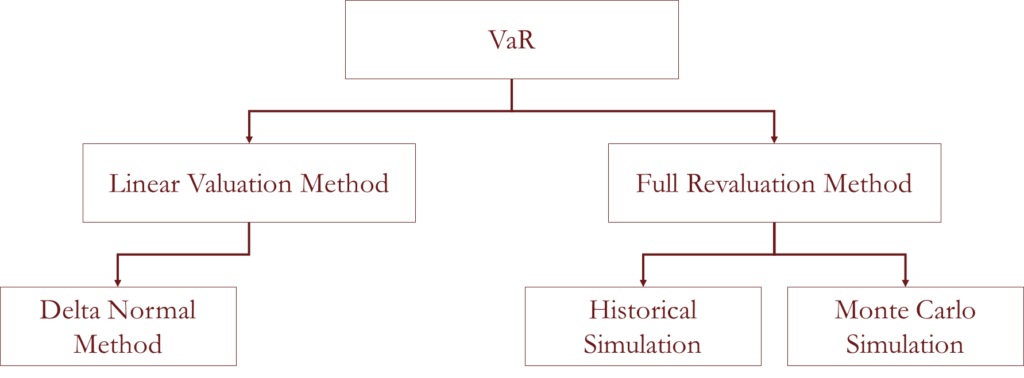
VaR Measurement Methods

VaR Measurement Methods – Linear Derivatives

• A linear portfolio is linearly dependent on the changes in the values of its underlying variables. A simple example of a linear portfolio is one that consists of 100 shares worth USD 50 each. The change in the value of the portfolio (∆P) is linearly dependent on the change in the stock price ∆S:

∆”P”=100∆S

• Delta of a derivative is the change in price of the derivative to change in the price of the underlying asset. The value of the delta for linear derivatives is constant for any change in the underlying.

1. The method to calculate VaR for linear assets is called Delta Normal method

2. Delta Normal method assumes that the variables are normally distributed

VaR Measurement Methods – Non-Linear Derivatives

• Linear Derivatives (e.g. forwards and futures) have Payoff  diagrams that are linear or almost linear.

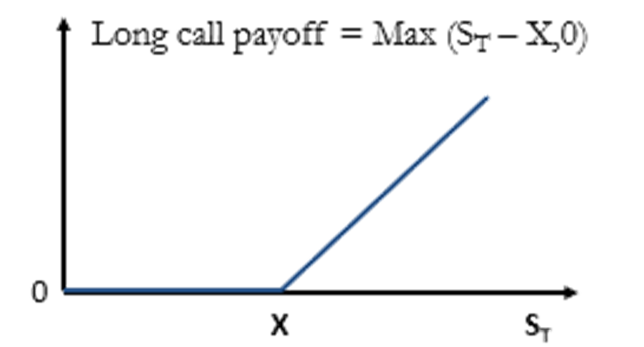
• Portfolios containing more complicated securities are not necessarily linear. Consider, for example, a portfolio consisting of a call option on a stock.

1. The payoff from the option is non- linear (Left Figure)

2. Prior to maturity, the option price is also a non-linear function of the stock price (Right Figure).

This means that there is not a linear relationship between the change in the portfolio value and the change in the stock price.

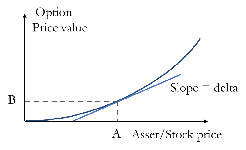
• The value of the delta keeps on changing with the change in the underlying asset for non-linear derivatives. So, delta-normal method cannot be used as they assume the linear payoff of the assets. The second term of this Taylor series approximation captures the curvature of the nonlinear derivative in addition to the slope or delta.

• To calculate the VaR for non-linear assets, full revaluation of the portfolio needs to be done. Monte Carlo methods or Historical Simulation are commonly used to fully revaluate the portfolio.

• To calculated the VaR using the delta-normal method, a linear approximation can be created. Even though this approximation is an imperfect proxy for the portfolio. It is computationally easy but may be less accurate. So approximately

∆P=δ∆S

where ∆P is the change in the price of the derivative, ∆S is the change in the price of the underlying asset, and δ is the delta of the derivative.

Historical Simulation

• Historical simulation involves identifying market variables on which the value of the portfolio under consideration depends. These market variables typically include equity prices, commodity prices, interest rates, credit spreads, volatilities, and so on. The market variables are usually termed risk factors.

• Daily data is collected on the behavior of the risk factors over a period in the past. It is assumed in this section that the past period is one from the immediate past. They are sorted out in an order and the VaR is calculated accordingly.

• Suppose the portfolio’s historical data is as given in the table.

Day	Stock Price (USD)	Exch. Rate USD/EUR	Int. Rate (%)	Cred. Spr. (bp)	…		…	Port. Val. (USD mill.)
0	50	1.2000	2.52	50	…		…	72.1
1	52	1.2012	2.54	53	…		…	72.5
2	46	1.2015	2.55	54	…		…	70.4
…	…	…	…	..	…		…
…	…	….	…	…	…		…
498	60	1.2520	2.30	48
499	60	1.2550	2.32	46	…		…	75.3
500	63	1.2500	2.36	47	…		…	76.3

• The portfolio under consideration is assumed to depend on many risk factors. The first four are a stock price, an exchange rate, an interest rate, and a credit spread. The interest rate is expressed in percentage terms, whereas the credit spread is expressed in basis points.

• It is assumed that today is Day 500, and it is important to know what might happen between today and tomorrow (i.e., between Day 500 and Day 501). The data given in the table is used to create 500 scenarios. (501 days of data is required to produce 500 scenarios because the changes are from one day to the next.). The table shown previously is an extract from the most recent 501 days (labeled Day 0 to Day 500) of historical data. 

• In practice, risk factors are divided into two categories –

1. Those where the percentage change in the past is used to define a percentage change in the future. For example, stock prices and exchange rates.

2. Those where the actual change in the past is used to define an actual change in the future. For example, credit spreads and interest rates.

• Table given in the next page is produced at the next stage of the historical simulation.

Scenario	Stock Price (USD)	Exch. Rate	Int. Rate (%)	Cred. Spr. (bp)	…	…	Port. Val. (Million $)	Loss (Million $)
1	65.52	1.2625	2.38	50	…	…	76.8	-0.5
2	55.73	1.2503	2.37	48	…	…	71.7	4.6
…	…	…	…	…	…	…	…	…
…	…	…	…	…	…	…	…	…
499	63.00	1.2530	2.34	45	…	…	75.3	1.0
500	66.15	1.2450	2.40	48	…	…	76.7	-0.4

• In the first scenario, it is assumed that all the risk factors behave between Day 500 and Day 501 in the same way as they did between Day 0 and Day 1. The stock price increased by 4% between Day 0 and Day 1. For the first scenario that is constructed, It is therefore assumed that it also increases by 4% between Day 500 and Day 501 so that the Day 501 stock price is $65.52 (63×1.04). Similarly, the exchange rate increased by 1% between Day 0 and Day 1. It is therefore assumed to also increase by 1% between Day 500 and Day 501 so that the Day 501 exchange rate is 1.2626 (1.2500×1.01).

• Meanwhile, the interest rate increased from 2.52% to 2.54% between Day 0 and Day 1. Thus, for the first scenario, it is assumed that the increase between Day 500 and Day 501 is same so that the Day 501 interest rate is 2.38%(2.36%+0.02%). Similarly, the credit spread can be calculated between day 500 and 501.

• The values of the risk factors for the second scenario (between Day 501 and Day 502) are calculated similarly using the changes that took place between Day 1 and Day 2. The third scenario is similarly calculated from the changes between Day 2 and Day 3, and so on. To complete the last two columns of the table (Portfolio value and Losses), it is necessary to produce portfolio values for each of the scenarios and then to calculate losses

• After creating scenarios, the losses are sorted from the largest to the smallest (as shown in the table in next page). The VaR with a 1-day time horizon and a 99% confidence level will therefore be the fifth worst loss because the fifth worst loss defines the loss that is at the first percentile point of the distribution (5/500=0.01).

•The expected shortfall is usually calculated as the average of the four losses that are worse than the VaR level. The VaR is USD 3.9 million, and the expected shortfall is –

(7.8+6.5+4.6+4.3)/4 = 5.8

Scenario Number	Loss (USD millions)
210	7.8
195	6.5
2	4.6
23	4.3
48	3.9
367	3.7
235	3.5
…	…
…	…
…	…

Portfolio Valuation

• A full revaluation of the portfolio for each of the scenarios can be computationally time consuming. One way of speeding up these calculations is to use Greek letters. The most important Greek letter is delta, and it is defined as:

δ = ∆P/∆S

where,

∆S is a small change in the risk factor.

∆P is the resultant change in the portfolio.

δ or Delta  is the rate of change in the value of the portfolio with respect to rate of change in the risk factor.

• EXAMPLE – Suppose the risk factor corresponds to a stock price and the delta of the portfolio with respect to that stock price is USD 50,000. This means that the value of the portfolio increases (decreases) by USD 50,000 for each USD 1 increase (decrease) in the stock price. If the stock price increased by USD 3.2, for example, we would estimate a USD 160,000 increase in the portfolio value. In general, the change in the portfolio value arising from the change ∆S  in a risk factor is ∆P=δ∆S.

• When there are many risk factors, it is necessary to calculate the effect of the change in each one and add them together. Suppose that

1. δ_i is the delta with respect to the i^th risk factor

2. ∆S_i is the change in the i^th risk factor for the scenario being considered.

The change in the portfolio value is then:

• EXAMPLE – Suppose the stock price, exchange rate, interest rate, and credit spread are the only risk factors. The deltas calculated for the risk factors (respectively) are 0.5, 20, -10, and 0.1 (measured as millions of USD per unit of the risk factor). Suppose changes in the four risk factors are –7.27, +0.03, +0.01, and +1 (respectively for the stock price, exchange rate, interest rate, and credit spread), the estimated change in the portfolio value is

(-7.27)×0.5+0.03×20+0.01×(-10)+1×0.1=-3.035

or a loss of about USD 3.0 million. For a linear portfolio, delta provides an exact answer. For non-linear portfolios, the change in the portfolio value given by delta is approximate.

• The calculation for a non-linear portfolio can be made more accurate by using another Greek letter that measures the curvature in the relationship between the portfolio value and risk factors. This letter is called Gamma and a better approximation of ∆P is thus:

Where γ is the gamma of the risk factor.

•When there are several risk factors (and each part of the portfolio depends on only one of them) the approximation becomes

A more complicated expression involving cross gammas is necessary for situations where there are portfolio components that are dependent on several risk factors.

Stressed Measures

• In the previous example, the data used to develop scenarios was from an immediately preceding period. However, bank regulators have moved to using what are termed stressed VaR and stressed expected shortfall for determining bank capital requirements. These are measures based on data from a one-year period that would be particularly stressful for a bank’s current portfolio. For example, March 2008 to February 2009 could be chosen by a bank that would be badly impacted by a crisis like the one experienced in 2007–2008.

• The scenarios are calculated from the percentage or actual changes that took place during the stressed period. Typically, 250 scenarios (produced from one year of data) are used rather than 500 scenarios (produced from two years of data). Everything else about the calculations remains the same. For example, if the percentage change in an exchange rate during a day in the stressed period was 5%, the scenario corresponding to that day would assume a 5% change in the exchange rate between today and tomorrow.

Delta-Normal Model

• As explained in portfolio valuation, equation given below is an exact result in the case of a linear portfolio and an approximate result for non-linear portfolios –

• To accommodate both types of risk factors which has been discussed in historical simulation, it is convenient to rewrite the above equation as –

In the case of risk factors where percentage changes are considered, x_i =(ΔS_i)/S_i  and a_i = δ_i S_i. In the case of risk factors where actual changes are considered, x_i = ΔS_i, and a_i = δ_i

• The mean (μ_p) and standard deviation (σ_P) of ΔP can be calculated as –

where μ_i, and σ_i, are the mean and standard deviation of x_i, (respectively) and ρ_ij is the coefficient of correlation between x_i, and x_j.

• If it is assumed that the change in the portfolio value is normal, it is easy to calculate either VaR or expected shortfall. As discussed, VaR is –

μ_p + σ_p U

Meanwhile, expected shortfall is –

where X is the confidence level and U is the point on the normal distribution that has an X probability of being exceeded.

• The change in the value of a linear portfolio is normally distributed if each of the x_i, is normal. This means that for a risk factor such as an equity price, the return over the period considered is normal. For a risk factor such as an interest rate, it means that the changes are normal.

• A common assumption is that the mean change in each risk factor is zero and therefore the average change in a linear portfolio is also zero. The assumption is not exactly true, but it is reasonable when considering short time periods. This assumption simplifies the expression for VaR to –

σ_P U

Meanwhile, the expression for expected shortfall simplifies to –

Limitations of Delta-Normal Model

• The  delta-normal  model  works  well  for  linear  portfolios  when  the  risk  factor  probability distributions  are  at  least  approximately  normal.  For  non-linear  portfolios,  it  will  only  give  an approximation. If  the curvature is small, the linear model is a reasonable approximation. But as curvature becomes larger, this is no longer true.

Monte Carlo Simulation

• Another  way  to  calculate  VaR  and  expected  shortfall  is  to  use  Monte  Carlo  simulations.  This approach is very similar to the use of  historical simulations, but with one key difference: Monte Carlo simulations generate scenarios by taking random samples from the distributions assumed for the risk factors (rather than using historical data). Monte Carlo simulations work for both linear and non-linear portfolios.

• Suppose that we assume the risk factor changes have a multivariate normal distribution (as in the delta-normal model). The procedure is as follows –

1. Value the portfolio today using the current values of  the risk factors.

2) Sample once from the multivariate normal probability distribution for the Δ〖x郢〗_i The sampling  should  be  done  in  a  way consistent  with  the  assumed  standard  deviations  and correlations (usually estimated from historical data). As we indicated earlier, for risk factors such as equity prices and exchange rates, the ∆𝑥_i  are percentage changes; for risk factors such as interest rates and credit spreads, they are actual changes.

3) Use the sampled values of  the Δx_i  to determine the values of  the risk factors at the end of the period under consideration (usually one day)

4) Revalue the portfolio using these risk factor values

5) Subtract this portfolio value from the current value to determine the loss

6) Repeat steps 2 to 5 many times to determine a probability distribution for the loss

• Suppose  that  there  are  total  of  1000  Monte  Carlo  simulation  trials.  The  VaR  with  a  99% confidence  level  for  the  period  considered  will  be  the  tenth  worst  loss  and  the  expected shortfall is the average of  the nine losses worse than this. As with other methods for calculating VaR and expected shortfall, the period considered when the simulation is carried out is usually one day and the square root of  time rule is used to convert the measure with a one-day time horizon to the corresponding measure with a T-day time horizon.

• The  Monte  Carlo  approach  assumes  that  there  is  a  known  probability  distribution  for  the risk factors. The usual implementation of Monte Carlo assumes a stable, Joint-Normal distribution for the risk factors. This is the same assumption used for Parametric VaR. The analysis calculates the covariance matrix for the risk factors in the same way as Parametric VaR.

• Unlike Parametric VaR, Monte Carlo Simulation –

1. Decomposes the covariance matrix and ensures that the risk factors are correlated in each scenario.

2. The scenarios start from today’s market condition and go one day forward to give possible values at the end of  the day.

Full, nonlinear pricing models are then used to value the portfolio under each of  the end-of-day scenarios.

For bonds, nonlinear pricing means using the bond-pricing formula rather than duration.

For options, it means using a pricing formula such as Black-Scholes rather than Greeks.

Monte Carlo Simulation – Advantage and Disadvantage

• Some of the advantages of Monte Carlo simulation are –

1. Unlike  Parametric  VaR,  it  uses  full  pricing  models  and  can  therefore  captures  the  effects  of nonlinearities.

2. Unlike Historical VaR, it can generate an infinite number of  scenarios and therefore test many possible future outcomes.

• Some of the disadvantages of Monte Carlo Simulation are –

1. The calculation of  Monte Carlo VaR can take 1,000 times longer than Parametric VaR because the potential price of  the portfolio has to be calculated thousands of  times.

2. Unlike Historical VaR, it typically requires the assumption that the risk factors have a Normal distribution.

Correlation Breakdown

• Not surprisingly, standard deviations increase during stressed market conditions. Interestingly, it is also true that correlations generally increase. It is sometimes stated that “in stressed markets all  correlations  go  to  one.”  This  is,  of  course,  an  exaggeration,  but  the  phenomenon  that correlations increase in stressed markets appears to be real. For example, during the 2007–2008 crisis,  default  rates  on  mortgages  in  all  parts  of  the  United  States  increased  together.  When there is a flight to quality in bond markets, the credit spreads of  all bonds throughout the world tend to rise together.

• The key point here is that in periods of  heightened volatility correlations can be quite different from  those  in  normal  market  conditions.  This  is  sometimes  referred  to  as  a  correlation breakdown. It does have significant implications for risk managers. When calculating VaR or ES they are concerned with estimating what will happen in extreme market conditions. They should, therefore, try and estimate what correlations will be in such conditions rather than what they are in normal market conditions.

Worst Case Analysis

• Occasionally,  when  there  are  repeated  trials,  an  analyst  will  calculate  statistics  for  worst-case results.  For  example,  if  a  portfolio  manager  reports  results  every  week,  he  or  she  might  ask what the worst result will be over a period of 52 weeks. If  the distribution of  the returns in one week is known, a Monte Carlo simulation can be used to calculate statistics for this worst- case result. For example, one can calculate the expected worst-case result over 52  weeks, the 95^th percentile of  the worst-case result, and so on.

• However, these worst-case statistics should not be regarded as an alternative to VaR and ES. They  are  only  appropriate  in  the  (relatively unusual)  situation  where  there  are  repeated  trials. Even then, risk  managers should  be interested  in aggregate  results  for a whole  period  rather than the statics of  the results over sub-periods.