Introduction to VaR

• VAR represents maximum potential loss in value of  a portfolio of  financial instruments with a given probability over a certain time horizon. In simpler words, it is a number that indicates how much a financial institution can lose with a given probability over a given time horizon.

EXAMPLE –

• If  the 95% daily VAR of  the assets is $100 million, then it means that out of  100 days there would be 95 days (or simply 95% of  the time), when the daily loss would be less than or equal to $100 million. This implies that for 5 days (or simply 5% of  the time), the daily loss will be more than $100 million.

• PS – There may be a day out of  100 when the loss is $5 billion, which means VAR doesn’t tell anything about the extent to which the loss can occur.

Confidence (x%)	z_(x%)
90%	1.28
95%	1.645
97.5%	1.96
99%	2.328

• When mean is 0, and return distribution is assumed to be normal, then

Dollar VaR_x%   = Percentage (%)VaR_x% × Portfolio Value

⇒ Dollar ($)VaR_x%   = z_x% × σ × Portfolio Value

• Also

n-day VaR = 1-day VaR×n

• For a two asset portfolio

Methods for Estimating VaR

• Linda Allen’s approaches for estimating VaR involve either a historical based approach or an implied volatility-based approach.

I. Historical based Approach

1. Parametric Approach

a) Exponential smoothing [Risk Metrics (EWMA model with λ=0.94)]

b) GARCH

c) Delta-normal VAR

2. Non-Parametric Approach

a) Historical Simulation

b) Multivariate Density Estimation

c) Hybrid Approach

II. Implied Volatility based Approach

1. Black Scholes Formula

Parametric Approaches

• The parametric approaches make some specific assumptions regarding the asset returns distribution. A parametric model typically assumes asset returns are normally or lognormally distributed with time-varying volatility.

• Data is used more efficiently with parametric methods than nonparametric methods.

Volatility

• A constant volatility is easy to estimate using historical data. But in practice, volatility changes through time. This leads to situations where asset returns tend to have fatter tails than a normal distribution would predict. This is important for the estimation of risk measures (such as VaR and expected shortfall) because these measures depend critically on the tails of asset return distributions.

• An alternative to assuming asset returns are constantly normal is to assume they are normal conditioned on the volatility being known.

1. When volatility is high, the daily return is normal with a high standard deviation.

2. When the volatility is low, the daily return is normal with a low standard deviation.

The conditionally normal model may not be perfect, but it is an improvement over the constant volatility model.

• To implement the conditionally normal model, it is necessary to monitor volatility so that a current volatility estimate is produced. Two models used for this purpose are – EWMA

model and the GARCH (1,1) model.

Deviations From Normality

• There are three ways in which an asset’s return can deviate from normality.

1. The return distribution can have fatter tails than a normal distribution.

2) The return distribution can be non-symmetrical.

3) The return distribution can be unstable with parameters that vary through time – This situation can lead to either of the first two situations.

When markets become stressed, volatility tends to increase. As markets calm, volatility tends to decrease.

• To illustrate the fat-tails phenomenon, let’s consider a variable X to be a mixture of two normal distributions. During a certain period, X has

1. A 50% chance of being normal with a mean of zero and a standard deviation of σ_1, and

2. A 50% chance of being normal with a mean of zero and a standard deviation of σ_2.

The probability density function is therefore a weighted average of two normal probability density functions:

• This figure plots this mixed distribution and compares it with the density function for a normal distribution (with the same standard deviation) when σ₁ = 0.5 and σ₂ = 1.5.

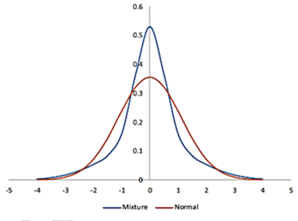
• The mixture distribution has the same characteristics as the distribution for the returns on the S&P 500.

• Because the mixed distribution is fat-tailed, there is more probability mass in the tails of the distribution.

• Also, the mixed distribution is more “peaked” than the normal distribution.

• An unstable mean can also lead to a non-normal distribution. The means of distributions can change through time for several reasons.

• The impact of the mean changing through time can be illustrated in the same way as the impact of the volatility changing through time. Combining a stochastic mean with a stochastic volatility can give rise to a non-symmetrical distribution. Consider a mixture of two normal distributions: The first has a mean of 0.3 and a standard deviation of 0.5, whereas the second has a mean of 1.5 and a standard deviation of 2.0. The resulting distribution will be skewed.

• The impact of volatility changing through time is quite important. For daily data, the volatility is much more important than the mean return. In fact, the mean daily return can be approximated to zero.

Unconditional and Conditional Normality

• To understand how fat tails are created by a stochastic volatility (i.e., a volatility that changes through time in an unpredictable way), it is important to distinguish between a model where returns are unconditionally normal and a model where they are conditionally normal.

1. In a model where returns are unconditionally normal, the probability distribution of the return each day has the same normal distribution with the same standard deviation.

2. In a model where the return is conditionally normal, however, the return distribution is normal each day, while the standard deviation of the return varies throughout time. During some periods it is high; during other periods it is low. This leads to an unconditional distribution with fat tails.

• When data on daily returns is collected, the unconditional distribution with fat tails is observed rather than the conditional distribution.

• Volatility can be monitored to estimate a conditional distribution for daily return.

Slow Changes Versus Regime Switching

• It is often reasonable to suppose that volatility changes slowly. Generally, large changes on either side tend to be followed by large changes, and small changes tend to be followed by small changes.  When volatility is high, large positive and negative changes in the price of an asset is observed. When volatility is low, the positive and negative changes are much lower.

• Sometimes, volatility changes abruptly. For example – Due to an unexpected event, volatility might jump suddenly from 1% to 3% per day. When markets calm down, it could suddenly jump back to 1% per day. This phenomenon is referred to as regime switching. Regime switches present additional challenges for risk managers because they are usually unanticipated. Models that have been working well may suddenly stop working well because the economic environment has changed.

Measurement of Volatility

• A rough definition is that the volatility of a variable measures the extent to which its value changes through time. In risk management, volatility of an asset is the standard deviation of its return in one day. If the return on day i is r_i and the asset provides no income, then

where S_i is the value of the asset at the close of trading on day i.

The usual formula for calculating standard deviations from sample data would give the volatility estimated from the return on the m previous days as:

where r ̅ is the average return over the m previous days, i.e.

In risk management, this formula is simplified in two ways: m – 1 is replaced by m, and,

 r ̅  is assumed to be 0.

• The two simplifications lead to the formula:

• Square of the standard deviation is defined as the variance rate. The formula which has been produced shows that the variance rate is the average of squared returns.

Day	Return
1	+1.1%
2	-0.6%
3	+1.5%
4	-2.0%
5	+0.3%
6	+0.4%
7	+1.8%
8	-0.3%
9	-0.3%
10	-0.4%

Estimating The Current Volatility

• There are dangers when trying to estimate volatility using the previous formula.

1. If m is too large, the estimate of the current volatility will not be reliable because it will use data from too long ago. If m=250, for example, volatility is estimated from daily data collected over one calendar year. If the volatility is cyclical (as it often is), it could be much lower (or higher) during the first six months than it is today. The calculated estimate would then not reflect current volatility.

2. With a smaller value (e.g., m=10 or m=20), the data being used is more relevant to estimating current volatility. However, the resulting volatility estimate may not be very accurate because it only uses a small number of data points.

3. Outliers or extreme values will lead to sudden changes. Suppose there was a large (positive or negative) return 25 days ago and the volatility is calculated using 50 days of data (m=50). For the next 25 days the large return will be included in the sample, and we will tend to get a high volatility as a result. In 26 days, however, the large observation will drop out of the data set, and the volatility will experience a large one-day decline as a result.

Exponential Smoothing

• Exponentially Weighted Moving Average (EWMA) can be used to overcome these problems. This approach was used by Risk Metrics to produce estimated volatilities of a wide range of market variables in the early 1990s.

• The previous formula gives equal weight to the squared returns in the sample (i.e., there are m squared returns and the weight given to each squared return is 1/m). The idea behind EWMA is that while the total of the weights given to all the squared returns must add up to one, the weights themselves do not have to be equal.

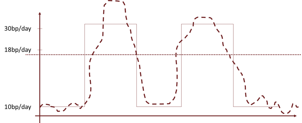
• In EWMA, the weight applied to the squared return from k days ago is λ multiplied by the weight applied to the squared return k-1 days ago (where λ is a positive constant that is less than one). Suppose w₀ is the weight applied to the most recent return (i.e., the return on day n-1). The weight for the squared return on day n–2 is λw₀; the weight applied to the squared return on day n–3 is λ² w₀; and so on. They decline exponentially one goes further back in time.

DAY	SQUARED RETURN	WEIGHT
n-1	r_(n-1)^2	w_0
n-2	r_(n-2)^2	λw_0
n-3	r_(n-3)^2	λ^2 w_0
n-4	r_(n-4)^2	λ^3 w_0
..	..	..
..	..	..

• The best value of λ is the one that produces the estimate with the lowest error. Risk Metrics found that setting λ=0.94 proved to be a good choice across a range of different market variables in the 1990s.

• λ is called ‘Persistence factor’ or even “Decay Factor”. Higher λ gives more weight to older data (impact of older data is allowed to persist). Lower λ gives higher weight to recent data (i.e. previous data impacts are not allowed to persist).  Higher λ means higher persistence or lower decay.  Since, (1- λ) is weight given to latest square return, it is called ‘Reactive factor’.

• The previous formula provides a very simple way of implementing EWMA. The new estimate of the variance rate on day n is a weighted average of:

1. The estimate of the variance rate made for the previous day (n-1), and

2. The most recent observation of the squared return (on day n-1).

• The weight given to the most recent variance estimate is λ and the weight given to the new squared return is 1-λ. The formula  is sometimes referred to as adaptive volatility estimation because prior beliefs about volatility are updated by new data.

• An attractive feature of the formula is that very little data needs to be stored once EWMA has been implemented for a particular market variable. Indeed, it is only necessary to store the most recent volatility estimate and even the return history does not need to be remembered. When a new return is observed, the volatility estimate is updated, and the new return can then be discarded.

Exponential Smoothing – Example

• Using a daily RiskMetrics EWMA model with a decay factor λ = 0.95 to develop a forecast of the conditional variance, which weight will be applied to the return that is 4 days old?

A. 0.000

B. 0.043

C. 0.048

D. 0.950

Correct Answer : B

Determining λ

• Risk Metrics used λ=0.94. This was an estimate produced in the 1990s and may not be appropriate to use today. However, a much higher or lower value of λ may also be inappropriate.

• If a much higher value of λ (e.g., 0.995), it would make EWMA relatively unresponsive to new data. From the previous formula, yesterday’s variance rate estimate would be given a weight of 99.5%, while the new squared return estimate would be given a weight of only 0.5%. Even several days of high volatility would not move the estimates much. Setting λ equal to a low number (e.g., 0.5) would lead estimates that overreact to new data. The estimates would themselves be too volatile.

• The 0.94 estimate found by Risk Metrics creates a situation where volatility estimates react optimally to new data. It should be noted that Risk Metrics wanted a λ that could be used for all market variables. If it had allowed itself the luxury of using different λs for different market variables, some of the λs used might have differed from 0.94.

Exponential Smoothing – Weights and Lambda

Garch

•The GARCH model can be regarded as an extension of EWMA. In EWMA, some weight is given to the most recent variance rate estimate and some weight is given to the latest squared return. In GARCH (1,1), some weight is also given to a long run average variance rate. The updated formula for the variance rate is

Here, V_L is the long run average variance rate.

The parameters α, β, and γ are the weights given to the most recent squared return, the previous variance rate estimate, and the long run average variance rate (respectively). Because the weights must sum to one:

α + β < 1

and

γ = (1 – α – β)

where α and β positive, and the unconditional variance has been normalized to one.

• It can be clearly observed that EWMA is a particular case of GARCH (1,1) where

γ = 0, α = 1-λ and β = λ.

• Both GARCH (1,1) and EWMA can be classified as first-order autoregressive models (or AR(1) models), because the value forecast for the variable (variance rate in this case) depends on the immediately preceding value of the variable.

• The (1,1) in GARCH (1,1) indicates weight is given to one (most recently observed) squared return and one (most recent) variance rate estimate. In the more general GARCH (p,q), weight is given to the most recent p squared returns and the most recent q variance rate estimates. GARCH (1,1) is by far the most widely used version of GARCH. The weights in a GARCH (1,1) model decline exponentially in the same way that the weights in EWMA decline exponentially.

• It is usual to define ω=γV_L, so  that

Since α + β + γ = 1

⇒V_L = ω/(1 -α -β)

Mean Reversion in Garch

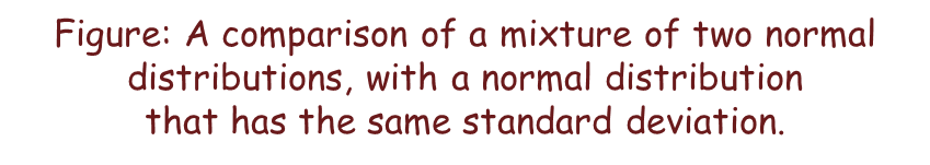
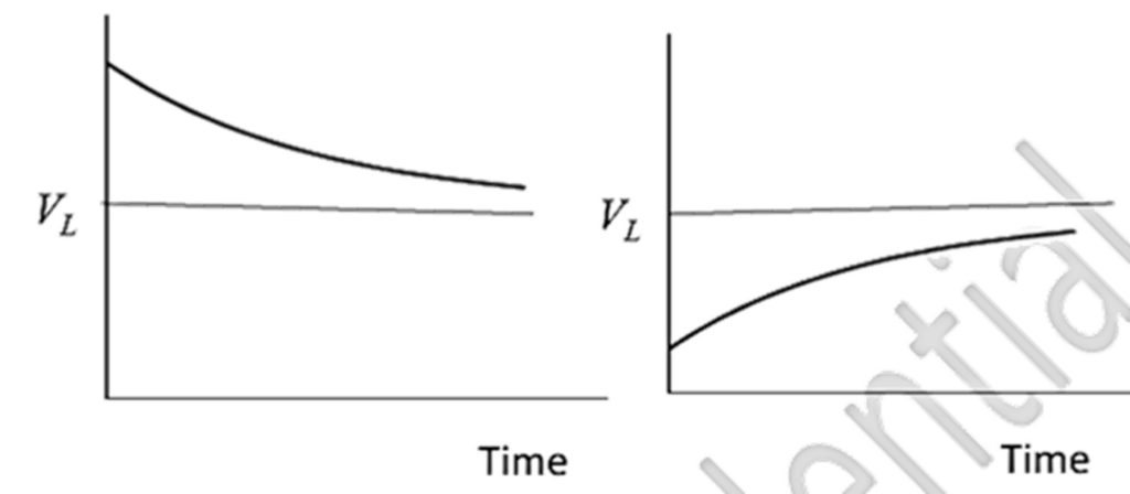
• The difference between EWMA and GARCH(1,1) is that in GARCH (1,1), the V_L term provides a “pull” toward the long-run average mean. In EWMA, however, there is no pull because this term is not included. This figure illustrates the pull.

a) When volatility is above the  long run average mean, it tends to be pulled down toward it.

b) When the volatility is below the long run average mean, it tends to get pulled up toward it.

Of course, this is just a tendency. The observed returns will lead to ups and downs superimposed on the average path given by the V_L term.

Mean Reversion

• This “pull” is referred to as mean reversion. GARCH(1,1) incorporates mean reversion whereas EWMA does not. It is important to note that mean reversion is a reasonable property for some market variables, but not for others. If the market variable is the price of something that can be traded, it should not exhibit a predictable mean reversion because otherwise there would be a market inefficiency which can be exploited for profit.

• A volatility is not the price of something that can be traded. There is, therefore, nothing to stop volatility exhibiting mean reversion. Indeed, there is every reason to suppose that it does. For example, when volatility becomes unusually high or low, we do not expect that to  last forever. It will eventually revert to normal levels. The same argument can be used for an interest rate. An interest rate is not the price of a traded security. Interest rates can therefore follow mean reversion and in practice appear to do so.

Garch Example

• Suppose a GARCH model is estimated from daily data as follows –

σ_t+1² = .000005 + 0.12μ_t² + 0.85σ_t²

Suppose that on a particular day ‘t’; actual return was -1% and the volatility (standard deviation) estimate for that was 1.8%. Calculate the volatility estimate for next day (t+1) and long-term average volatility (to which the model shows reversion over-time).

• Which of the following GARCH models will take the shortest time to revert to its mean ?

A. h_t= 0.05+0.03r_t-1²+0.96h_t-1

B. h_t= 0.03+0.02r_t-1²+0.95h_t-1

C. h_t= 0.02+0.01r_t-1²+0.97h_t-1

D. h_t= 0.01+0.01r_t-1²+0.98h_t-1

Long Horizon Volatility

• If a conditional normal model is assumed, the one-day volatility can be used to provide a normal distribution for the change in a market variable. This can be used as an input to the delta-normal model for determining the one-day VaR . If volatility is constant, it is reasonable to assume that the variance rate over T days is T times the variance rate over one day. This means that the volatility over T days is √T times the volatility over one day. This square root rule corresponds to a well-known rule that uncertainty increases with the square root of time.

• Mean reversion suggests a possible improvement to the square root rule.

a) If the current daily volatility is high, it can be expected to decline. That means the square root rule based on the current daily volatility overstates VaR.

b) Similarly, if the current daily volatility is low, it can be expected to increase and so the square root rule will tend to understate VaR.

The same phenomenon applies to expected shortfall.

• It can be shown that under GARCH (1,1), the expected variance rate on day t is given by

This formula can be used to calculate the average variance rate over the next T days.

Non-Parametric Approaches

• In the nonparametric approaches, there are no underlying assumptions of the asset returns distribution, and hence it is less restrictive Three main nonparametric methods used to estimate VaR are: (1) historical simulation, (2) hybrid approach, and (3) multivariate density estimation.

• The nonparametric have the following advantages over parametric approaches –

1. Nonparametric models do not require assumptions regarding the entire distribution of returns to estimate VaR.

2) Issues like fat tails, skewness, and other deviations from any assumed distribution (like a normal distribution) don’t hinder the VaR estimation process for nonparametric methods.

3) Multivariate density estimation (MDE) takes into account the current market environment, hence making it more relevant.

4) Multivariate density estimation (MDE) can also introduce dependence on economic variables.

Alternative Weighting Scheme – MDE

• In EWMA, the weights applied to historical data decline exponentially as one moves back in time. In an alternative method, sometimes referred to as multivariate density estimation (MDE), another approach is used to determine weights. With MDE, an analysis is carried out to determine which periods in the past are most similar to the current period. Weights are then assigned to a day’s historical data according to how similar that day is to the current day.

• Consider interest rates. The volatility of an interest rate tends to vary according to interest rate levels. Specifically, volatility tends to decrease as rates increase. In calculating the volatility of an interest rate, it can make sense to give more weight to data from periods where the level of interest rates is similar to current interest rates levels and allow the weight for a day’s data to taper off as the difference between the interest rate levels for that day and the current day increases.

• Sometimes several state variables (referred to as conditioning variables) are used to determine how similar one period is to another. For example, GDP growth could be used in conjunction with interest rate levels as conditioning variables for interest rate volatility. When there are several conditioning variables (X₁, X₂, …, X_n) the similarity between today and any previous day can be determined by calculating a metric such as:

where

X_i^∗ is the value of X_i today, (X_i ) ̂ is the value of X_i on the day from history being considered, and a_i is a constant reflecting the importance of the i^th variable. The more similar a historical day is to the current day, the smaller this metric becomes.

DISADVANTAGES –

• MDE may lead to over-fitting of data while identifying required assumptions regarding the weighting scheme and determining the number of observations used to estimate volatility.

• MDE requires a large amount of data.

Historical Simulation – Example

• Consider the following data where ordered simulated price returns of an asset are given as below for sample of 500 days and the asset is trading at 70. What is the VaR at 99% confidence if the returns for the last 500 days are –

-7%, -6.7%,-6.6%, -6.5%,-.6.1%,-5.9% … 4%, 4.75%,5.1%, 5.2%,5.3%

Hybrid Approach

Return	Periods Ago	Hybrid Weight	Cum Hybrid Weight	HS Weight	Cum HS Weight
-3.3	3	0.022144839	0.022144839	0.01	0.01
-2.9	2	0.022596774	0.044741613	0.01	0.02
-2.7	65	0.006328331	0.051069944	0.01	0.03
-2.5	45	0.009479113	0.060549057	0.01	0.04
-2.4	5	0.021267903	0.08181696	0.01	0.05
-2.3	30	0.012834429	0.09465139	0.01	0.06

Implied Volatility

• The implied volatility of a one-month option gives an indication of the average volatilities expected over the next month, the implied volatility of a three-month option gives an indication of what volatilities are expected to be over the next three months, and so on. Because volatilities exhibit mean reversion, we do not expect implied volatilities to be the same for options of all maturities.

• Options are not actively traded on all assets. This means reliable implied volatilities for an asset are sometimes not available. Nevertheless, risk managers should monitor implied volatilities as well as volatilities calculated from historical data whenever possible.

• One closely monitored implied volatility index is the VIX. This is an index of the implied volatilities of 30-day options on the S&P 500. Typical values for the index are in the 10 to 20 range (indicating a 30-day volatility for the S&P 500 of 10% to 20% per year). During October 2008 (in the midst of the crisis), the VIX index reached 80 (indicating an implied volatility of 80% per year and 5% per day) on two occasions.

Correlation

• It is important for risk managers to monitor correlations as well as volatilities. When the delta-normal model is used to calculate VaR or expected shortfall for a linear portfolio, correlations between daily asset returns (as well the daily standard deviations of asset) are needed.

• To update correlation estimates, rules similar to those which were used for updating volatility estimates can be applied. Just as updating rules for volatility work with variances, the updating rules for correlations work with covariances. If the mean daily returns are assumed to be zero, the covariance of the returns between two variables is the expectation of the product of the returns. The EWMA model for updating the covariance between return X and return Y is

where

cov_n is the covariance estimated for day n and

x_n and y_n are values of x and y on day n (respectively).

• The correlation between two variables is their covariance divided by the product of their standard deviations. If EWMA has been used to estimate the standard deviations of the returns, the coefficient of correlation can be estimated. For consistency, the same value of λ should be used for updating both variance rates and covariances.

• Suppose the volatility of X and Y are estimated for day n-1 as 1% and 2% per day (respectively) while the coefficient of correlation has been estimated as 0.2. The covariance is the coefficient of correlation multiplied by the product of the standard deviations:

COU_n-1 = 0.2 x 0.01 x 0.02 = 0.00004

• Suppose that the returns observed on day n-1 for X and Y are both 2% and we use a value for λ of 0.94. The covariance is updated as follows:

COU_n-1 = 0.94 x 0.00004 +(1 – 0.94) x 0.02 x 0.02 = 0.0000616

• With the same value of λ the volatilities of X and Y are updated to ____1.086%______and ______2%_____ (respectively) and the new coefficient of correlation is

0.0000616/0.01086 x 0.02 = 0.28

• GARCH (1,1) can also be used to update a covariance. However, using GARCH to update multiple covariances in a consistent way is quite complex.