Machine Learning And Prediction

Learning Objectives
- Explain the role of linear regression and logistic regression in prediction.
- Understand how to encode categorical variables.
- Discuss why regularization is useful, and distinguish between the ridge regression and LASSO approaches.
- Show how a decision tree is constructed and interpreted.
- Describe how ensembles of learners are built.
- Outline the intuition behind the K nearest neighbors and support vector machine methods for classification.
- Understand how neural networks are constructed and how their weights are determined.
- Evaluate the predictive performance of logistic regression models and neural network models using a confusion matrix.
- Video Lecture
- |
- PDFs
- |
- List of chapters
Chapter Contents
- Introduction
- Dealing with categorical variables
- Regularization
- Regularization – ridge regression
- Regularization – lasso
- Regularization – elastic net
- Difference between ridge regression and lasso
- Regularization – example
- Decision trees
- Decision trees – information gain
- Decision trees – threshold
- Decision trees – example
- Decision trees – overfitting
- Ensemble techniques
- Ensemble techniques – bootstrap aggregation
- Ensemble techniques – random forests
- Ensemble techniques – boosting
- K-nearest neighbors
- Support vector machines
- SVM extensions
- Logistic regression
- Logistic regression – example
- Model evaluation – continuous variable
- Model evaluation – category variable
- Neural networks
- Neural network – example
Introduction
- Categorical variables are an important category of variables in statistics. It is crucial to handle such variables appropriately. Because they arrange data based on some qualitative feature, these variables are sometimes known as qualitative variables.
- Linear regression is an essential statistical method for understanding the dependency pattern in data. However, having too many parameters might confuse the model, therefore it should be ensured that the model only contains the most significant parameters. The regularization approach is employed for this. It is a parameter reduction strategy used when the model has a large number of strongly linked variables.
- Logistic regression is yet another useful statistical technique. It aids in categorizing the observations into one of two outcomes.
Dealing with categorical variables
- Dummy variables are an essential type of categorical variable. Any qualitative data to be incorporated into a regression or machine-learning model must be quantified. This technique of converting non-numerical data into numbers is also known as mapping or encoding.
- Qualitative information can be of the following two types –
- Naturally Unordered – For example, information on geographical regions – Pacific, Rocky Mountain, Midwest, Northeast, and South.
- Naturally Ordered – For example, information on company size – small, medium and large.
- To manage naturally unordered information, it is preferable to utilize a different dummy variable (0-1 dummy) for each category. This process is known as one-hot encoding. However, the dummy variable trap should be avoided. For example, for five geographical regions in the above example of naturally ordered data, four 0-1 dummies could have been used.
- To manage naturally ordered information, however, a single dummy variable can be used. For example, for large, medium, and small business sizes, a single dummy that assumes a value of 0 for small firms, 1 for medium firms, and 2 for large firms can be added.
Regularization
- It is critical to ensure that models do not get too vast or complicated, since these models can no longer make sense and the parameter estimations can become offsetting with one another, where one parameter may have an opposite impact than the other.
- The regularization method can be used to solve this problem. It is a technique used to prevent overfitting by adding a penalty term to the loss function. The loss function is already explained in the previous chapter. The penalty term discourages the model from learning complex relationships that may not generalize nicely to new data. It encourages the model to have smaller weights, thereby reducing its complexity.
- It may be applied to both regression and machine-learning models. However, before regularization, the data must be either normalized or standardized.
- Regularization has the following advantages –
- It simplifies the models.
- It makes them easier to comprehend.
- It decreases the chance of overfitting the training sample.
- The two regularization procedures are as follows –
- Ridge Regression – The penalty term in this regression is the sum of the squares of the coefficients.
- Least Absolute Shrinkage and Selection Operator (LASSO) – The penalty term in this regression is the sum of the absolute values of the coefficients.
Regularization – ridge regression
- Ridge regression is also called L2 regularization. This ensures that, for a pair of correlated variables, a large positive coefficient is not assigned to one and a large negative coefficient is not assigned to another. For a data set containing n observations for m different features and the output variable y, the objective (Loss) function for a ridge regression is given as –
- The first component of the objective function is the standard residual sum of squares for regression, while the second is a shrinkage factor that penalizes large-slope parameter values. Only after sufficient trial and error can the suitable value of λ be determined. It is the hyperparameter since it is not included in the model.
where
λ is the parameter that controls the relative weight given to the shrinkage versus model fit.
α ̂ and β ̂i are the model parameters.
Regularization – lasso
- LASSO is also known as L1 regularisation. LASSO penalises the parameter in the same way as ridge regression does, however instead of the square of the parameters, it penalizes the absolute values.
- This method is commonly known as the feature selection technique since it aids in the removal of inconsequential features. If the value of λ is increased further, more features are lost.
Regularization – elastic net
- Elastic net is a mix of the Ridge regression and the LASSO, with the loss function containing both squared and absolute-value parameters functions.
- By carefully selecting the hyper-parameters, the benefits of both ridge and LASSO may be realized by lowering the magnitudes of some parameters and deleting some minor features completely.
Difference between ridge regression and lasso
- Although both LASSO and ridge regression are employed to regularize the model, the two have important distinctions. As a result, the choice of one strategy over another is situational. If the goal is to lower the extreme parameters, ridge regression should be employed; if the goal is to totally eliminate specific features from the model, LASSO should be utilized.
- Some differences between the ridge regression and LASSO are given in the table below –
| Ridge Regression | LASSO |
| The values of α and β can be found analytically | The values of α and β can be found only using numerical methods |
| Tends to reduce the magnitude of the β parameters, making them closer to, but not equal to, zero. | It sets some of the less-important β estimates to zero. |
Regularization – example
- Table given below records the parameters of OLS regression for the data from the PCA example of the last chapter. Since the magnitudes of observations are similar, rescaling of the data can be skipped.
- It is clear from the table that ridge regressions decrease the size of the parameters, with a larger value of λ decreasing them even more. In contrast, LASSO decreases certain coefficient values to zero. Only one coefficient (plus the intercept) is non-zero when λ= 0.1.
- This example suggests that regularization is effective if the hyper-parameters are selected carefully and it should –
- be easily interpretable
- produce accurate forecasts
- Sometimes, the simpler models produced using regularization generalize better than the original OLS linear regression model.
| Feature | OLS | Ridge, α = 0.1 | Ridge, α = 0.5 | LASSO, α = 0.01 | LASSO, α = 0.1 |
| Intercept | 5.17 | 2.67 | 2.46 | 2.61 | 2.39 |
| USTB1M | -23.22 | -6.55 | -2.00 | -1.13 | 0 |
| USTB3M | 50.64 | 10.00 | 2.45 | 1.35 | 0 |
| USTB6M | -37.64 | -3.82 | -0.51 | 0 | 0 |
| USTB1Y | 11.00 | 0.70 | 0.40 | 0 | 0 |
| USTB5Y | -5.55 | -1.75 | -1.41 | -1.22 | -0.71 |
| USTB10Y | 9.13 | 0.57 | -0.11 | 0 | 0 |
| USTB20Y | -5.88 | -0.08 | 0.36 | 0.14 | 0 |
Decision trees
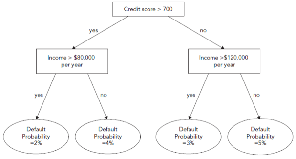
- A supervised machine-learning method called a decision tree may be used to assess input features progressively. It is shown as a tree with a question at each node, branching out to other nodes or leaves (end). It may be used for both classifying and estimating values for continuous variables and is also called classification and regression trees (CART). These models are regarded as white boxes since they are easy to comprehend (interpretability). Below is an example of a decision tree to determine a borrower’s creditworthiness.
Building a decision tree requires taking into account a metric known as information gain of a feature. This is a gauge of how much ambiguity is eliminated by learning more about the characteristic. Each node’s characteristic enhances information gain. Entropy and the Gini coefficient are the two metrics for information gain that are most frequently utilized.
Decision trees – information gain
- Two measures of information gain are –
- Entropy – It is a measure of disorder and by construction, it lies between 0 and 1. It is defined as –
- Gini – It can be calculated as –
- Gini and entropy usually lead to very similar decision trees.
where M is the total number of possible outcomes and pi is the probability of that outcome.
Decision trees – threshold
- Another important aspect of decision trees is the Threshold. A threshold in decision trees is a value that divides the data into two or more subgroups based on the value of a feature. To generate the most effective decision tree, the decision tree algorithm chooses the appropriate threshold to split the data at each node.
- Consider a decision tree that is used to determine if an animal is a cat or a dog based on its weight. The algorithm may conclude that a weight threshold of 10 pounds is the optimum way to divide the data into two groups, with animals weighing less than 10 pounds classified as cats and animals weighing more than 10 pounds classified as dogs.
- The threshold value is significant since it establishes the decision tree’s decision bounds. The decision tree algorithm tries to select the threshold value that results in the optimal separation of the classes.
Decision trees – example
- A risk manager wants to find out the firms that will pay or not pay dividends over the next year and plans to construct a model to predict it. For this, he assumes four binary variables -
- Whether the dividend was paid last year – 1 for yes and 0 for no
- Whether the firm’s earnings have dropped last year – 1 for yes and 0 for no
- Whether it is a large-cap stock – 1 for yes and 0 for no
- Whether it is in the tech sector – 1 for yes and 0 for no
- Also, a variable for the percentage of retail investors constituting the shareholder base is included. The table on the next page highlights these features for a sample of 20 firms.
- If a specific question provides a flawless division across categories, it would be considered highly useful and is regarded as a pure set. For instance, supposing dividends were paid on all technology equities will lead to a pure set. The worst-case scenario, on the other hand, would be if exactly half of the technology companies paid dividends and the other half did not. In this instance, knowing a company’s status as a tech stock or not would be of considerably less help.
- First, the Gini coefficient for the output variable, Dividend, is measured before incorporating any information about other features. Out of 20, 12 firms have paid dividends, hence –
- This acts as a base level with which the fall in the Gini coefficient is compared as the tree grows.
- Step 1 – Selecting root node. A feature is selected for the root node. The feature selected is such that the Gini coefficient falls the most and is found using trial and error. Here it is Large cap.
- From the table, 13 firms are large cap and out of these 11 paid dividends. Hence, the Gini is –
- Among 7 firms that are not large cap, 1 paid a dividend while 6 did not. Hence –
- Weighted Gini is then –
- Similar computations for earnings drop and tech will result in information gains of 0 and 0.003, respectively. The threshold value for binary variables is determined by the decision tree algorithm itself but to find the threshold that optimizes information gain for retail investors, an iterative process is required. It turns out that for all potential threshold values, the information gain for retail investors is smaller than 0.225. As a result, the Large cap serves as the decision tree’s root node.
| Data point | Dividend | Earnings drop | Large cap | Retail investor | Tech | Data Point | Dividend | Earnings Drop | Large Cap | Retail Investor | Tech |
| 1 | 1 | 0 | 1 | 40 | 1 | 11 | 0 | 0 | 0 | 20 | 1 |
| 2 | 1 | 1 | 1 | 30 | 0 | 12 | 0 | 0 | 1 | 70 | 0 |
| 3 | 1 | 1 | 1 | 20 | 0 | 13 | 1 | 1 | 0 | 30 | 1 |
| 4 | 0 | 0 | 0 | 80 | 1 | 14 | 1 | 0 | 1 | 70 | 0 |
| 5 | 1 | 0 | 1 | 20 | 1 | 15 | 1 | 0 | 1 | 50 | 1 |
| 6 | 0 | 1 | 0 | 30 | 1 | 16 | 1 | 0 | 1 | 60 | 1 |
| 7 | 0 | 1 | 0 | 40 | 0 | 17 | 1 | 1 | 1 | 30 | 0 |
| 8 | 1 | 0 | 1 | 60 | 0 | 18 | 0 | 1 | 0 | 30 | 1 |
| 9 | 1 | 1 | 1 | 20 | 1 | 19 | 0 | 0 | 0 | 40 | 0 |
| 10 | 0 | 1 | 1 | 40 | 0 | 20 | 1 | 1 | 1 | 50 | 0 |
And
- At subsequent nodes, features are chosen in a similar way to maximize Gini. Note that the tree does not need to be symmetrical. A possible final tree is shown in the figure given below.
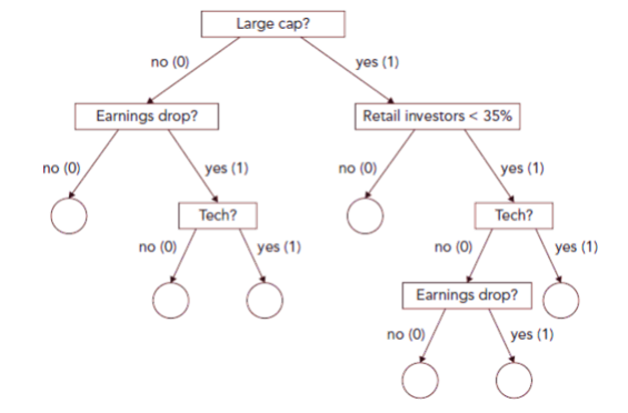
- For large-cap stocks the most important next feature is the proportion of retail investors. It turns out that a threshold of 35% is optimal for this feature at this node of the tree.
- This iterative approach to growing the tree in the way described in the previous example is known as the Iterative Dichotomizer algorithm. The tree is completed when either a leaf is reached that is a pure set (The left leg ends in a pure set) or all the features have already been used so that the data cannot be split further (The right leg ends due to features exhaustion). Creating a perfect classification is impossible in the previous example, so although some branches end in a pure set, others do not.
Decision trees – overfitting
- When data have many features, decision trees can suffer from overfitting. However, it can be prevented using the following two techniques -
- Stopping rules – Specifying stopping rules prior to tree building involves stating that only a certain number of branches can be made before stopping and placing leaves.
- Pruning – When the rule is that splitting stops when the number of training set observations corresponding to a node that is reached is below a certain number. This is referred to as pre-pruning. Post-pruning involves constructing a large tree and then removing the “weakest” nodes.
Ensemble techniques
- Constructing ensembles of learners involves using a range of different models and combining their outputs into a single metamodel. This has two objectives -
- Through the “wisdom of crowds” and a result somewhat like the law of large numbers, model fit can be improved by making many predictions and averaging them;
- The techniques aim to build in protections against overfitting. Ensembles combining weak learners with the best model often perform better than the latter on their own.
- Although ensembles could involve combining any type of machine-learning models, the approach is straightforwardly explained using decision trees as an illustration. Three important ensemble techniques -
- Bootstrap aggregation
- Random forests
- Boosting
Ensemble techniques – bootstrap aggregation
- Bootstrap aggregation or bagging is the process of creating numerous decision trees using the training sample as a starting point and then combining the resulting predictions or classifications to form a new prediction or classification. A basic bagging algorithm for a decision tree involves the following steps -
- Sample a subset of the complete training set.
- Construct a decision tree in the usual fashion.
- Repeat steps 1 and 2 many times, sampling with replacement so that observation in one subsample can also be in another subsample.
- Average the resulting forecasts.
- As a result of the replacement sampling used for the data, some observations won’t show up at all. In that replication, the observations that were not chosen (referred to as out-of-bag data) will not have been utilized for an estimate; nonetheless, they can be used to assess the performance of the model.
- Pasting is similar to bagging in that sampling occurs without replacement. Pasting with 100,000 items in the training set and sub-samples of 10,000 results in a total of 10 sub-samples.
Ensemble techniques – random forests
- An ensemble of decision trees where the observations or features are sampled without replacement is called a random forest. During sampling, the average number of features picked is the square root of the total number of features available. A single tree’s predictions may be suboptimal, but the combined influence of numerous trees enhances the forecast. When the individual model outputs have minimal correlations with one another, the performance enhancements are highest.
Ensemble techniques – boosting
- Boosting is the process of attempting to increase a model’s performance by training it on the mistakes of its predecessors. The two main variations of boosting are -
- Gradient boosting – It builds a new model based on the residuals of the prior one, which becomes the target. In other words, the labels in the training set are substituted with the preceding iteration’s residuals, which serve as a surrogate for the gradient.
- Adaptive boosting (AdaBoost) – It involves training a model with equal weights on all observations and then incrementally increasing the weight on misclassified outputs to incentivize the classifier to focus more on those situations. Boosting differs from bagging in that each bootstrap model is built in a similar manner.
K-nearest neighbors
- It is a simple and intuitive, supervised machine-learning model used to classify or predict the values of a target variable. To predict an observation, not in the training set, K observations are searched in the training set that is closest to it using either Euclidian or Manhattan distance. KNN is a lazy learner because it learns the relationships slowly compared to other approaches.
- The steps involved in a typical KNN implementation are as follows -
- A distance measure (Euclidean or Manhattan) and a value of K are selected.
- For each data point in the training sample, K nearest neighbours are identified in the feature space to the point in the feature space for which a prediction is to be made.
- Simply said, the KNN algorithm searches the feature space for the K nearest data points to the new data point that has to be classified or forecasted. The user determines the value of K, which specifies the number of nearest neighbours to be examined. After identifying the K nearest neighbours, the method predicts the class or value of the new data point based on the majority class or mean value of the K neighbours.
- Consider a dataset including consumer information such as age, income, and spending patterns. Further, assume that the aim is to predict if a new consumer will buy a product or not. To utilise KNN, first, a suitable value for K is chosen, say K=5. Then five customers are picked who are the most similar to the new client in terms of age, income, and spending patterns. If three of the five neighbours bought the product, the algorithm predicts that the new client would do the same.
- Although KNN is a simple and effective technique, it can be computationally costly when dealing with huge datasets. Furthermore, choosing the optimal value of K can be difficult, and the technique might be sensitive to the distance metric used to quantify the similarity between data points.
Support vector machines
- A group of supervised machine learning models called SVMs are excellent for classification tasks involving a lot of features. An SVM’s goal, when a sample with two characteristics is taken into account, is to discover the location of a line that would divide the sample into two groups. The same space is then used to map new data points that are not in the sample and forecast which of the two groups they will belong to.
- An SVM constructs the widest path consisting of two parallel lines, separating the observations into two separate groups. The data points that lie on the edge of the path are known as the support vectors. The centre of the path is used as the separation boundary.
- For example, suppose a retail bank is interested in developing a machine-learning model that would make car loan decisions on a case-by-case basis. The information on the customers’ income, savings, and whether the loan was granted for a balanced sample of 12 prior applicants is given in the table on the next page.
- It turns out that the widest pathway has as its center –
-12.24+0.90×Monthly income×1.26×Total savings=0
with the two edges –
-12.24+0.90×Monthly income+1.26×Total savings=1
-12.24+0.90×Monthly income+1.26×Total savings=-1
| Applicant number | Monthly income (USD 000s) | Total savings (USD 000s) | Loan granted? (yes = 1; no = 0) |
| 1 | 2.5 | 5.0 | 0 |
| 2 | 1.8 | 0.5 | 0 |
| 3 | 4.1 | 1.6 | 0 |
| 4 | 0.8 | 2.0 | 0 |
| 5 | 6.2 | 4.0 | 0 |
| 6 | 3.8 | 6.2 | 0 |
| 7 | 2.1 | 9.0 | 1 |
| 8 | 4.6 | 10.0 | 1 |
| 9 | 1.8 | 13.0 | 1 |
| 10 | 5.2 | 8.0 | 1 |
| 11 | 10.5 | 3.0 | 1 |
| 12 | 7.4 | 8.5 | 1 |
- The fitted decision boundary, the support vectors, and the data points are plotted in the figure given below.
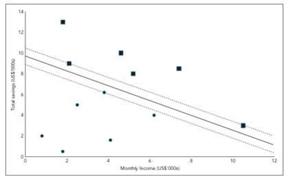
- The edges of the widest path is represented by the dotted line and its centre by the solid line.
SVM extensions
- Although the preceding example was rather straightforward, the underlying concepts and the framework for optimization would apply to any number of variables. When there are more features, a hyperplane with dimensions one fewer than the number of features is found instead of a line in the centre with the largest margin.
- Also, in contrast to the previous example, a perfect separation is not possible. It is then necessary to specify a tradeoff between the width of the path and the extent of misclassifications to which the path gives rise. Further extensions are available to allow for the path to be nonlinear.
Logistic regression
- Finance is full of scenarios where the model’s output is categorical with binary outcomes such as mortgage default and flagging fraudulent transactions, etc. For modelling the probability distributions of such variables, it may be tempting to assign a value of one to one outcome and a value of zero to another. Such linear models, however, are inefficient because they lack the ability to assure that the calculated probabilities are between zero and one, resulting in incorrect projections.
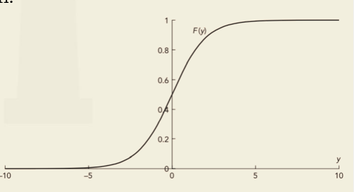
- Logistic regression or logit can be considered a better specification for modelling the probability distribution of these variables. In order to bind the outputs between zero and one, logit provides a cumulative logistic function transformation.
- This function results in a sigmoid shape as given in the figure below.
- For a linear regression model, the functional form of y_j when there are m features, is estimated as –
- The probability that yj=1 is given by –
- It is important to note that the parameters α and β_i cannot be estimated using OLS, because it is not linear. Hence, the maximum likelihood method is used. This selects the parameters that maximizes the chances of the training data occurring and takes the functional form of –
- The Π notation denotes that the functions are multiplied because the joint probability of all the n data points is the product of F(y) across the positive outcomes (1) in the training set multiplied by the product of (1-F(y)) across the negative outcomes (0), given they are independent. If yj is 1, the jth function reduces to F(yj ); for zero, it reduces to 1 – F(yj ).
- It is easier to maximize the log-likelihood function, log(L), than the likelihood function. This is given as –
- This can also be written as –
- After estimating the α and βs using maximum likelihood, a threshold, Z, is set for predictions from the model and the value of Pj is estimated. Finally, the category to which the jth observation belongs is specified using the following relationship –
- In cases where the cost of erroneously categorizing a value of y as 1 when it should be 0 is the same as the cost of incorrectly classifying it as 0 when it should be 1, the value of Z can be set to 0.5. However, in circumstances such as categorizing loans based on the likelihood of default (yj=1) and the likelihood of complete repayment (yi=0), Z can be adjusted to a smaller number, such as 0.05 for decision-making. This is because the cost of making a poor loan is far higher than the cost of the profit lost as a result of the loan not being made.
and the probability that yj = 0 is (1-Pj).
Logistic regression – example
- For a sample of 500 observations for the database of Lending Club which was a peer-to-peer retail lender, the dependent variable is the state of the loan which can be 0 (fully paid off) or 1 (deemed irrecoverable). The table given below shows the results.
- The non-linear nature of the logistic transformation makes the parameter estimates from a logit model non-interpretable. However, their signs and levels of statistical significance can still be examined. Two important takeaways from this example are –
- Borrowers with longer loan terms and those paying higher interest rates have a significantly higher probability of default, whereas those with a mortgage have a significantly lower probability of default.
- All other factors such as the total sum borrowed, instalment, etc., do not significantly affect the probability that borrowers will default on their loans.
- Ridge regression and LASSO can also be used with logistic regression. Maximizing the likelihood is equivalent to minimizing –
| Parameter | Definition | Estimate | Standard error |
| Bias term | The intercept | -5.3041 | 1.051 |
| Amount | Total sum borrowed | -0.0001 | 0.000 |
| Term | Length of the loan (months) | 0.0768 | 0.034 |
| Interest rate | APR charged (%) | 0.1147 | 0.045 |
| Instalment | Monthly instalment | 0.0025 | 0.004 |
| Employment history | Length of borrower’s employment history (years) | 0.0428 | 0.059 |
| Homeowner | 1 = owns home; 0 otherwise | 0.1149 | 0.409 |
| Mortgage | 1 = has a mortgage; 0 no mortgage | -0.9410 | 0.435 |
| Income | Annual income (USD) | -0.0001 | 0.000 |
| Delinquent | Number of times borrower has been more than a month behind with payments in the past two years | 0.0985 | 0.113 |
| Bankruptcies | Number of publicly recorded bankruptcies | -0.1825 | 0.361 |
Model evaluation – continuous variable
- For continuous outputs such as yield, forecast error aggregation measures are used to evaluate the model. Two such measures are –
- Mean Squared Forecast Error (MSFE) – It is the average of the squared deviations of true observations from the predicted observations. It is given as –
- Absolute Forecast Errors (AFE) – It is the average of the absolute deviations of true observations from the predicted observations. It is given as –
Where, yi is the true observation value, y ̂_i is the predicted value, and ntest is the test sample size.
Model evaluation – category variable
- Categorical outputs which are binary in nature can be evaluated through calculations based on a confusion matrix. The confusion matrix is a 2×2 table highlighting possible outcomes and the correctness of the predictions. As long as the outcome variable in a model is binary, this matrix will be the same 2×2 table irrespective of the number of features included, sample size and the type of model.
- Suppose a model is constructed to calculate the probability that a firm will pay a dividend in the following year or not based on a sample of 1,000 firms, of which 600 did pay and 400 did not. After translating the probabilities into 0-1 variable, the confusion matrix may take the following form.
- Correct predictions are always found on the leading diagonal while off-diagonal terms imply an incorrect prediction. From the previous example, four elements of the table can be identified. These are –
- True positive – The model predicted a positive outcome, and it was indeed positive. (TP)
- False negative – The model predicted a negative outcome, but it was positive. (FN)
- False positive – The model predicted a positive outcome, but it was negative. (FP)
- True negative – The model predicted a negative outcome, and it was indeed negative. (TN)
- These four elements help to specify many performance metrics. Some prominent ones are –
- Similar to the tradeoff between type I and type II errors in hypothesis tests, there is a tradeoff between the true positive and false positive (i.e., the true negative) rate when setting Z.
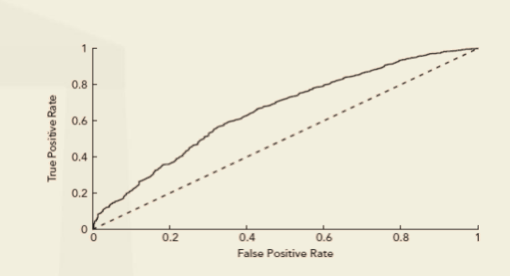
- The receiver operating curve (ROC) is a way of showing this link between true positives and false positives, Figure given below shows the ROC for different values of the threshold, Z.
- Area under the ROC curve (AUC) highlights the accuracy of predictions from the model.
- A completely accurate set of predictions gives an AUC of 1.
- An AUC value of 0.5 (dashed line) indicates that the model has no predictive ability.
- An AUC value less than 0.5 indicates that the model has a negative predictive value.
- Although the formulae for the performance metrics described above assumed only two possible outcomes, the formulae can be extended to situations where there are several classes.
| Prediction | |||
| Firm will pay dividend | Firm will not pay | ||
| Outcome | Pays dividend | 432 (43.2%) – TP | 168 (16.8%) – FN |
| No dividend | 121 (12.1%) – FP | 279 (27.9%) – TN | |
Neural networks
- Artificial neural networks (ANNs) are a type of machine-learning technique that is loosely based on how the brain computes. It has two important aspects -
- Feed-forward network – A feed-forward neural network is a sort of artificial neural network that only allows information to flow in one way, from input to output.
- Back-propagation – The backpropagation method works by propagating the error from the output layer to the input layer backwards across the network. This entails computing the derivative of the loss function with respect to each node’s weights and biases. To decrease error, the weights and biases are then changed using an optimisation process such as gradient descent.
- The figure shown above depicts a straightforward feed-forward network.
- Three input features, one hidden layer with three nodes, and one output variable, y, make up the neural network shown above. The hidden nodes’ values are computed from the input variables, and from the hidden nodes’ values, the value of y is calculated. The following are the equations that may be used to determine values at hidden nodes –
- ϕ in the previous equations are referred to as activation functions. The activation functions are applied to a linear function of the input feature values. The value of the target output variable y is calculated in a similar way from the values in the hidden layer –
- The connection between the inputs and outputs must be nonlinearized by these activation functions for the model to work; otherwise, it would just be a linear regression. As neural networks seek to identify complicated non-linear interactions, this would not be of relevance.
- A common activation functional form is the logistic (sigmoid) function from logistic regression. Biases are the constant components of the linear functions (w1, w2, w3, and w4) to which the activation functions are applied. Weights are the coefficients in the linear functions (w parameters). The training set and criteria used in logistic or linear regression are used to calculate these parameters. For predicting values of a continuous random variable, parameters are chosen to minimize the mean squared errors, while maximum likelihood criterion is used when neural networks are used for classification.
- The gradient descent algorithm is used to determine the best values of the parameters as there is no perfect analytical formula for this. This is a general algorithm for finding parameter values that minimize an objective function. It involves starting with trial values of the parameters and then determining the direction in which their values should change to best improve the value of the objective function. This can be thought of as the line of steepest descent down a valley. steps are taken down the valley along this line of steepest descent, a new line of steepest descent is calculated, another step is taken, and so on.
- The size of the step is known as the learning rate and is an important hyper-parameter. If the learning rate is too small, the gradient descent algorithm will take too long to reach the bottom of the multi-dimensional valley. If it is too large, it may oscillate from one side of the valley to the other.
- Often, there are several hidden layers and many more than three nodes per layer. This leads to a very large number of parameters and leads to a possibility of over-fitting. Over-fitting is avoided by carrying out calculations for the validation data set at the same time as the training data set.
- As the algorithm steps down the multi-dimensional valley, the objective function will improve for both data sets, but at some stage, further steps down the valley will start to worsen the value of the objective function for the validation set while improving it for the training set. This is the point at which the gradient descent algorithm should be stopped because further steps down the valley will lead to over-fitting.
- Interpreting or evaluating a neural network model is harder than for more conventional econometric models. It is possible to examine the fitted weights, looking for very strong or weak connections or where estimates are offsetting, which would be indicative of overfitting.
- Suppose a neural network is built using the same ten features and output as for the logistic regression example taken previously. The objective is to build a model to classify loans in terms of whether they turn out to default or repay. A single hidden layer feed-forward network with back-propagation is employed. It contains ten units in the hidden layer and a logistic activation function. The loss function is based on an entropy measure, and the optimization takes 297 iterations to converge.
- Given that the same data and features have been employed for both the logistic regression and neural network, the results from the models can be compared in the table given below.
- For simplicity, a threshold of 0.5 is employed, so that for any predicted probability of default greater than or equal to 0.5, the fitted value is of default, whereas if the probability is less than 0.5, the fitted value is of no default.
- The performance summary measures show that, as expected, the fit of the model is somewhat weaker on the validation data than on the training data. This result could be interpreted as slight over-fitting, and it might be worth removing some of the least empirically relevant features or applying regularization to the fitted models.
- Comparison also reveals that there is very little to choose between the two models. On the training sample, their accuracies are identical, and although the neural network performs better in terms of its precision, its recall is weaker. But when applied to the validation sample, the logistic regression does better on accuracy and precision grounds, but worse on recall. these contradictory indicators illustrate the importance of fitting the evaluation metric to the problem at hand.
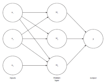
H1 = ϕ(w111x1 + w112x2 + w113x3 + w1)
H2 = ϕ(w121x1 + w122x2 + w123x3 + w2)
H3 = ϕ(w131x1 + w132x2 + w133x3 + w3)
y=ϕ(w211H1 + w221H2 + w231H3 + w4 )
Neural network – example
Training sample (500 data points) Validation sample (167 data points) Measure Logistic regression Neural network Logistic regression Neural network Accuracy 0.842 0.842 0.713 0.701 Precision 0.656 0.750 0.600 0.541 Recall 0.236 0.169 0.283 0.377 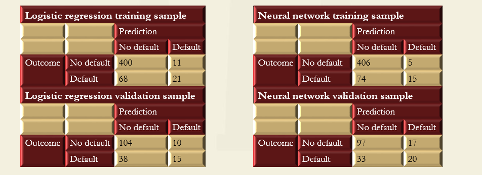
Go to Syllabus
Courses Offered
Popular Courses
FRM Part 1
FRM Part 2

By : Micky Midha
9 Hrs of Videos
Available On Web, IOS & Android
Access Until You Pass
Lecture PDFs
Class Notes

By : Micky Midha
12 Hrs of Videos
Available On Web, IOS & Android
Access Until You Pass
Lecture PDFs
Class Notes

By : Micky Midha
257 Hrs Of Videos
Available On Web, IOS & Android
Access Until You Pass
Complete Study Material
Quizzes,Question Bank & Mock tests

By : Micky Midha
240 Hrs Of Videos
Available On Web, IOS & Android
Access Until You Pass
Complete Study Material
Quizzes,Question Bank & Mock tests

By : Shubham Swaraj
Lecture Videos
Available On Web, IOS & Android
Complete Study Material
Question Bank & Lecture PDFs
Doubt-Solving Forum