
Learning Objectives
- Discuss the philosophical and practical differences between machine-learning techniques and classical econometrics.
- Explain the differences among the training, validation, and test data sub-samples, and how each is used.
- Understand the differences between and consequences of under fitting and over fitting, and propose potential remedies for each.
- Use principal components analysis to reduce the dimensionality of a set of features.
- Describe how the K-means algorithm separates a sample into clusters.
- Be aware of natural language processing and how it is used.
- Differentiate among unsupervised, supervised, and reinforcement learning models.
- Explain how reinforcement learning operates and how it is used in decision-making.
- Video Lecture
- |
- PDFs
- |
- List of chapters
Chapter Contents
- Introduction
- Difference Between ML and classical econometrics
- Advantages of ML over classical econometrics
- Sample splitting and preparation
- the problems of over-fitting and under-fitting
- Tradeoff between over-fitting and under-fitting
- Difference between over and under-fitting
- Tradeoff between over and under-fitting
- Data preparation
- Data Cleaning
- Types of machine learning
- Unsupervised learning
- Supervised learning
- Reinforcement learning
- Principal components analysis
- The k-means clustering algorithm
- performance measurement for k-means
- Selection of K
- k-means clustering – an example
- Disadvantage of k-means clustering
- Natural language processing
- Natural language processing – advantages
- Natural language processing – steps
- Reinforcement learning
- Reinforcement learning – an example
- Differences between different types of ML
Introduction
- Machine learning (ML) is a branch of artificial intelligence (AI) and computer science which incorporates a range of techniques that can be used to train a model to capture trends in the given data. These captured trends find application in prediction and classification.
- Machine-learning techniques were created primarily by engineers rather than statisticians; hence, distinct notations and terminology are commonly used.
- For example, independent variables are known as inputs or features, dependent variables are known as outputs or targets, and the values of these outputs are known as labels.
Difference Between ML and classical econometrics
The model development procedures and methods of specification check using Machine learning and classical econometrics differ significantly –
| Classical Econometrics | Machine Learning |
| Developed by statisticians | Created primarily by engineers |
| The variables are predetermined, and the data generation process is based on some economic or financial theory. | ML allows the data to choose the features (variables) that should be included in the model. |
| It requires well defined and structured data to work with | ML can work on complex and unstructured data |
| Typically, econometric modelling makes assumptions such as the regressors being independent and normally distributed. | In machine learning, such assumptions are not necessary. |
| The analyst decides on the variables to include in the model and tests the model. | The analyst does not test a particular hypothesis about the best model. |
| The major ways of evaluating traditional models are statistical significance, the goodness of fit, and error-term diagnostic testing, etc. | In supervised machine learning, these metrics are replaced with an emphasis on forecast accuracy. |
| The statistical models can be interpreted in the terms of simple relationships between variables. | The interpretation of ML models can be complex |
| R is one of the popular tools for analysis. | Python is one of the popular tools for analysis. |
Advantages of ML over classical econometrics
- There are significant advantages of machine learning techniques over traditional linear econometric approaches for prediction –
- Machine learning works well when there is little financial theory to guide the choice of variables to include in a model, or where the researcher is unsure whether a linear or nonlinear specification is more appropriate.
- The flexible functional forms employed in ML specifications imply that they can capture potentially complex interaction effects between variables.
- Machine learning can capture nonlinearities in the dependence of the dependent variable on each of the explanatory variables.
Sample splitting and preparation
- In conventional econometrics, it is common to retain part of a data sample for testing the fitted model and determining how well it can predict observations on the dependent variable that it has not seen. This leads to a distinction between in-sample (used for model estimation) and out-of-sample (sometimes known as a hold-out sample) parts of the data.
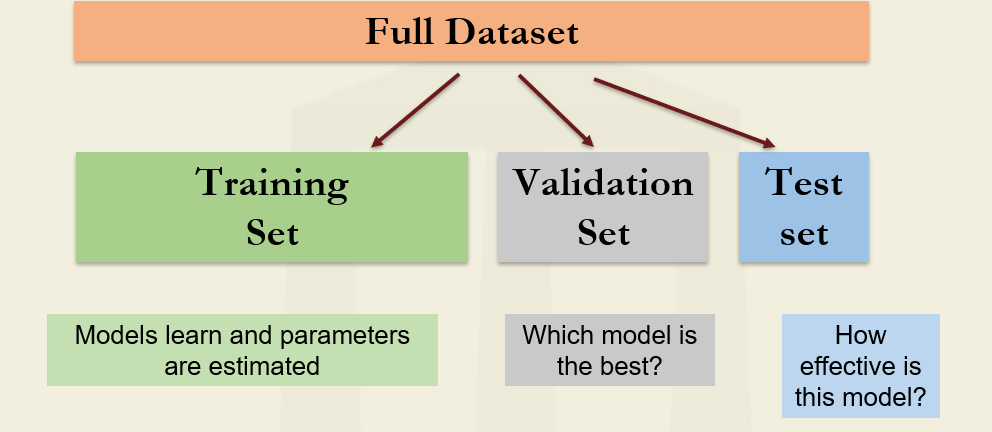
- Due to the heightened possibility for overfitting and the lack of an existing specification based on financial theory in ML approaches, the use of a hold-out sample is even more important. However, rather than two parts, the overall sample is usually split into three –
- Training set – The training set is employed to estimate model parameters (e.g., the intercept and slopes in a regression).
- Validation set – The validation set is used to select between competing models. Different alternative models are compared to determine which one generalizes best to new data.
- Testing set – Once the model selection is complete, the validation set is contaminated and no longer available for a truly independent test of the model’s performance. The test set is retained to determine the final chosen model’s effectiveness.
| Training set | Validation set | Test set |
| Used to estimate model parameters. | Used to select superior model from candidate set of models. | Validate the efficiency of the model selected. |
| Small training sample can lead to biased estimates of parameters | Small validation sample can lead to inaccurate model evaluation. | Small test set can lead to inefficient conclusion on the model effectiveness |
- A good model will be able to fit almost as well to the test sample as it did to the training sample because the machine has learned the critical elements of the relationships between the features and the output(s) without fitting to unimportant aspects (noise).
- There is no hard and fast rule for finding the size of each sample. Generally, when the sample size is big, around two-thirds of the sample is utilized for training, with the remaining third divided evenly between validation and testing.
- A small sample size for the training set can introduce biases in the parameter estimation, whereas if the validation sample is too small, model evaluation can be inaccurate which makes it hard to identify the best specification.
- Moreover, the sample selection criteria for different types of datasets are different –
- For cross-sectional data (data with no natural ordering), the three samples should be drawn randomly from the total dataset.
- For time-series data, it is common for the training data to be the first part of the sample, then the validation data, with the test data being at the end. This sample split has the advantage of allowing the model to be tested on the most recent data.
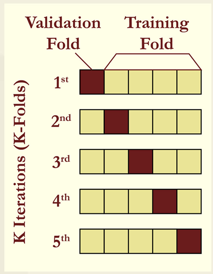
- Cross-Validation Searches-The whole dataset may not always be large enough to offer adequate training, validation, and test samples. Cross-validation can be used to solve this problem. It requires merging the training and validation data into a single sample and retaining only the test data. This merged data is then divided into equal-sized subsamples, with the estimate conducted again and one of the subsamples excluded each time.
-> M-fold cross-validation (also known as 𝑘-fold cross validation) is a well-known example of this technique. It divides the training and validation data into 𝑘sub-samples. The model is trained and evaluated 𝑘times. Commonly used values for 𝑘-fold cross-validation are 𝑘 5 and 𝑘 10. - Leave-one-out cross-validation-As k rises, the limit is 𝑘 𝑛, which corresponds to having as many folds as the entire number of data points in the training set. This is a special case of cross validation and is referred to as leave-one-out cross-validation.
the problems of over-fitting and under-fitting
- Over-fitting is a situation in which a model is chosen that is “too large” or excessively parameterized.
- An over-fitted model catches too much random noise in the training set apart from the main signal.
- Because the error rate on the training set is so low, over-fitting gives the impression of a great specification. But an over-fitted model will perform considerably worse on new data, and the model will be unable to generalize successfully.
- Under-fitting is the inverse of over-fitting and happens when important patterns in the data are missed by the model.
- For example, the relationship between hedge fund performance and size (as measured by assets under management) is slightly quadratic. A linear model would be unable to capture this behaviour making the model under-fitted. A better specification would permit a nonlinear relationship between fund size and performance.
- Another example of under-fitting is the failure to incorporate key interaction variables.
Tradeoff between over-fitting and under-fitting
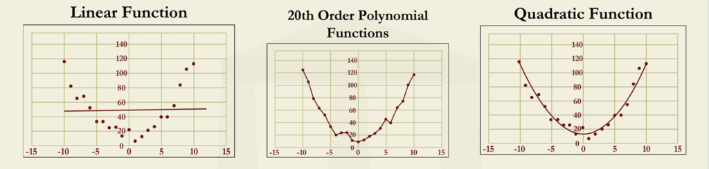
- The left panel shows a linear regression fit to the data, which is clearly insufficient to
describe the series and will give rise to predictions that are highly biased. - The center panel shows the result of applying a high-order polynomial fit. This line
contours perfectly with the training set but is evidently an overfit (high variance of errors). - The right panel shows a quadratic polynomial, which has the right trade-off between over
and under-fitting
The series of figures given above illustrates how under-fitting and over-fitting can manifest
themselves.
Difference between over and under-fitting
| Over-Fitting | Under-fitting |
| Model contains excessive parameters. | Model misses important patterns and interaction parameters. |
| Model catches too much random noise than only the pertinent signals. | Model estimates a monotonic connection between the relevant variables. |
| Model gives low bias predictions but with high variance. | Model gives biased predictions but with low variance. |
| It is a big problem in Machine learning. | It is a big problem in Classical econometrics. |
- Since machine learning incorporates a large number of parameters (even more than 1000 parameters), over-fitting is a more severe issue for machine learning than with classical econometric models.
- Under-fitting may appear to be a more persistent problem in traditional models than in alternative machine-learning techniques where no assumptions about the structure of the model are enforced. However, machine-learning algorithms also have the potential to underfit the data. This can occur when the amount or quality of inputs is inadequate, or when
anti-overfitting measures are very strict.
Tradeoff between over and under-fitting
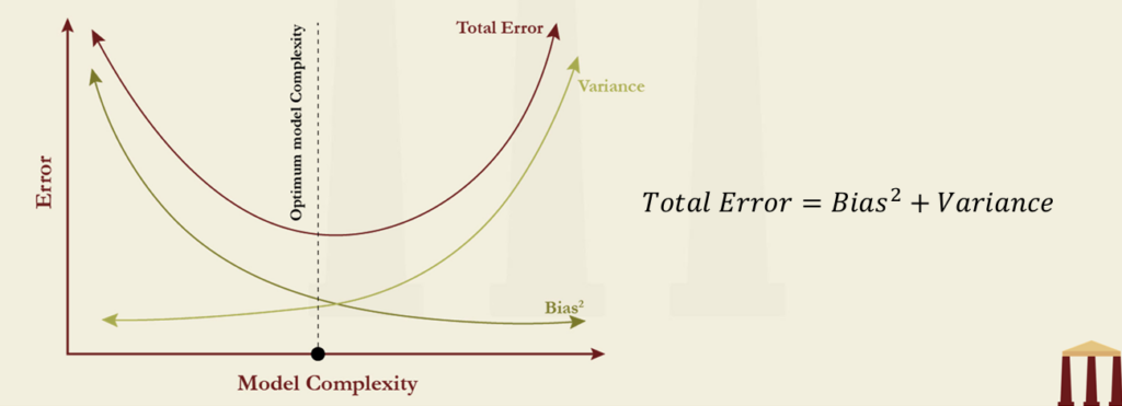
- The size of the machine-learning model is chosen with the help of bias-variance tradeoff.
- If the model is under-fitted, the omission of relevant factors or interactions will lead to biased predictions but with low variance.
- If the model is overfitted, there will be low bias but the high variance in predictions.
This is illustrated in this figure.
Data preparation
- Applying machine learning tools effectively to estimate the parameters requires all variables to be measured on the same scale. Rescaling can be done with the help of either
- Standardization or
- Normalization
- Standardization creates a scale for measuring the variable with zero mean and unit variance. This is similar to the process of transforming a variable into the standard normal variable.
- Normalization creates a variable that is bound between zero and one and may not have zero mean and unit variance.
- Except for the variables that are being predicted, it is important that all other variables are rescaled using either normalization or standardization for a given dataset.
- When the dataset contains outliers, standardization is preferred over normalization as normalization squashes the data points into a tighter range of 0 and 1 which is inconsistent with the original data.
Data Cleaning
- Large datasets have their own set of issues, such as duplicate observations or outliers. These must be addressed in order to properly utilise the data using machine learning techniques. The technique that attempts to resolve these difficulties is known as data cleaning, and it costs over 80% of the total project time. Data cleaning helps in eliminating the following issues –
- Inconsistent recording
- Unwanted observations
- Duplicate observations
- Outliers
- Missing data
- Outliers should be handled with care as they have the ability to alter the results significantly.
- Missing data is the most prevalent issue in datasets. If the amount of missing data is little, it can be discarded. But if it is considerable, any of the two procedures listed below can be used –
- Replace missing data on a feature with the mean or median of the remaining observations on the feature.
- Estimate missing data using observations from other features.
Types of machine learning
- Unsupervised Learning
- Supervised Learning
- Reinforcement Learning
The types of machine learning techniques are –
Unsupervised learning
- Unsupervised learning aids in the identification of patterns or trends in data via data clustering. It uses unlabeled data and there is no stated goal. It can uncover minimum yet relevant features with strong explanatory power.
- It may appear to be of little use because it is not used to create predictions, yet it may be incredibly beneficial in describing and comprehending a dataset’s structure.
- Banks, for example, must have a fraud detection model that may be used to identify and examine questionable transactions. The difficulty here is in identifying key factors. Unsupervised learning can aid in this situation by emphasizing the traits that may distinguish some transactions from others. These findings may then be used to improve the training and development of the fraud detection model.
- Some of the methods used in unsupervised learning are –
- Principal Component Analysis
- K-Means Clustering Algorithms
Supervised learning
- Supervised learning is useful for either predicting the value of a variable or classifying an observation. To do this, some labelled data must be supplied for the algorithm to learn from.
- Some possible applications of supervised learning in prediction are in –
- Time series – In the forecasting of gross national product or the value of the S&P 500 index next year.
- Cross-sectional series – In prediction for a data point that is not in the sample. For example, if an apartment is put up for sale, how much would it be worth?
- It finds its application in credit decisions for classifying potential borrowers according to whether they are acceptable credit risks. Important tools of supervised learning have been discussed in the next chapter in detail.
- Labeled data – It refers to data that has been labelled with one or more labels that indicate certain attributes or traits, classes, or included objects. In simple terms, it is created when relevant labels, tags, or classifications are applied to raw data that has been gathered.
Reinforcement learning
- Reinforcement learning employs a trial-and-error strategy that can greatly benefit in making a sequence of judgments in a dynamic environment.
- The best approach to acquire or sell a big block of shares, how to manage a portfolio, and how to hedge derivatives portfolios may all be determined using it in risk management.
- This has been discussed in detail in upcoming slides.
Principal components analysis
- An important tool in unsupervised learning is principal components analysis (PCA). This is a well-known statistical technique for dimensionality reduction. It is a way of creating a small number of variables (or components) that provide almost the same information as a large number of correlated variables. The number of principal components that are produced is equivalent to the number of variables in the initial dataset. The new components are uncorrelated from each other.
- PCA assumes that the variance of the features carries the information, meaning that features with higher variation carry more information. Therefore, PCA utilizes a linear transformation that preserves the maximum variance in the data using the minimum number of dimensions.
- The process of PCA involves detecting patterns in the data and constructing new variables, referred to as principal components, that capture the maximum amount of variation in the dataset. These principal components are created as linear combinations of the original variables. The first principal component captures the most variation, followed by the second, and so on.
- A very well-known example of PCA that has been discussed in the chapter “VRM 13 – Modeling Non-Parallel Term Structure Shifts and Hedging” of the FRM Part 1 curriculum. It is related to the reduction of a collection of yield-curve changes to a small number of explanatory variables or components. PCA seeks a limited number of uncorrelated variables that describe these changes. The observed changes should be a linear combination of the new variables.
- The most important explanatory variable for yield-curve changes is a parallel shift. The next important explanatory variable is a twist, in which short rates go one way and long rates move the other.
- When the actual motions are stated as a linear combination of the components, the first three components account for more than 99% of the variation. This is because the yield movements are highly correlated, and the majority of the information contained in them can be captured by a limited number of explanatory factors.
The k-means clustering algorithm
- The K-means algorithm is a straightforward, unsupervised algorithm to separate observations into clusters. It helps identify the structure of a dataset. The number of required clusters, K, is determined at the outset, and often, several different values of K are tried by the analyst. The
algorithm proceeds as follows –
- Randomly choose initial values for the K centroids, which are the centres of the clusters.
- Allocate each data point to its nearest centroid.
- Recalculate the centroids to be at the centres of all of the data points assigned to them.
- Repeat steps 2 and 3 until the centroids no longer change.
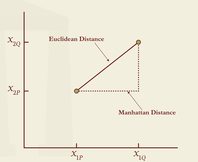
- Steps 2 and 3 require a definition of the distance of each observation to the centroids. There are two commonly used measures –
- The Euclidean (“as the crow flies”) distance – The Euclidean distance (𝐿2-norm), 𝑑E , between the two points is calculated as the square root of the sum of the squares of the
distances in each dimension. It is the direct route between two points. - The Manhattan distance measure – For two dimensions, the Manhattan distance(𝐿1-norm) between two points, is an approximation of the distance between two buildings that might be required when driving a car.
- Suppose two features, 𝒙𝟏, and 𝒙𝟐, have two observations on each of them, represented by the points 𝑃and 𝑄in the Figure given alongside. These have coordinates (𝑥 ,𝑥 ), and (𝑥 ,𝑥 ), respectively. The Euclidean distance, 𝑑 , between the two points would be calculated as –
- The Manhattan distance between 𝑃 and 𝑄 would be calculated as –
- If there were 𝒎 features for two points 𝑃 and 𝑄, the Euclidean distance is generalized as –
- Extending this to 𝒎 dimensions (𝒎features), the Manhattan distance is generalized as –
- The formulae discussed above describe the distance between one point 𝑃 and another point 𝑄. However, the purpose of 𝐾-means is not to minimize the distance between points, but rather to minimize the distance between each point and its centroid.
performance measurement for k-means
- The performance of 𝐾-means clustering depends on the collective closeness of data points to the centroids. In other words, the performance depends on how effectively the algorithm minimizes the distance between each data point and the centroid. This performance is measured in terms of a quantity defined as inertia(within-cluster sum of squares).
- If𝑑𝑗 is the distance between a data point 𝒋(j=1,…,n) and the centroid to which it has been allocated, we can define the inertia,𝐼, can be defined as-
- The lower the inertia, the better that cluster fits the data. When the 𝐾-means algorithm is carried out, the usual practice is to try several different initial values for the centroids. These sometimes result indifferent clusters. For a particular 𝐾, the best clustering is the one for which the inertia is least.
Selection of K
- In the same way that 𝑅2 will never fall when more explanatory variables are added to a regression model, the inertia will never rise as the number of centroids increases. In the limit, as 𝐾 reaches its maximum possible value of 𝑛, the total number of datapoints, so that each data point has its own cluster, the inertia will fall to zero. Such a model with 𝐾 𝑛 would clearly be of no value even though it would fit the data perfectly, and therefore, choosing K optimally is an important practical consideration.
- There are two popular approaches to finding the optimal value of 𝐾.
- Screen plot – In this approach, the value of 𝐼 is calculated for different values of 𝐾 and the results are plotted. The figure is then examined to find the elbow which is chosen as the optimal value of K. Elbow is an obvious point at which 𝐼 starts to decline more slowly as K is further increased. It is also used to select the number of components to use in PCA.
- Silhouette coefficient – This compares the distance of each observation from other points in its own cluster with its distance from points in the closest cluster. The best value of 𝐾 is the one that gives the highest silhouette score.
k-means clustering – an example
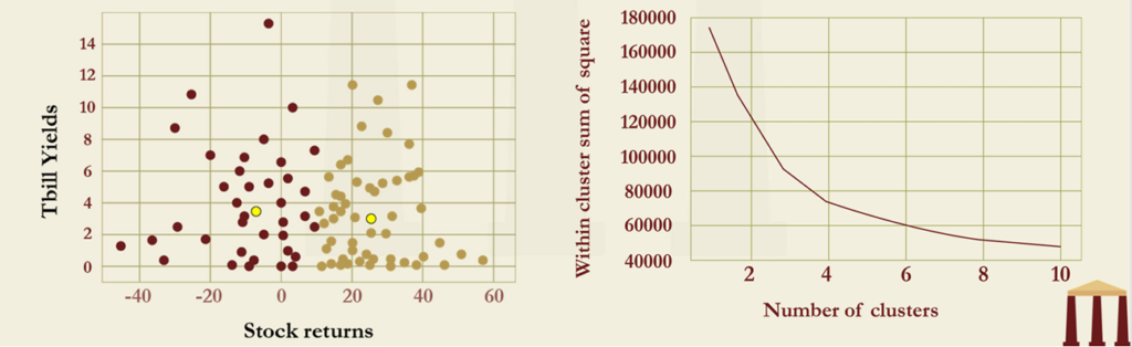
- The first figure shows the 𝐾-Means plot, with 𝐾 =2, applied to annual value-weighted stock index returns (all stocks on NYSE, Amex, and NASDAQ) and Treasury bill yields from 1927 to 2021. The fitted centroids are [-7.70, 3.51] and [25.42, 3.16]. The algorithm has identified two separate clusters based on separating the stock returns into “boom” and “bust” regimes.
- The optimal value of 𝐾 for this data is investigated in the right figure, which is a screen plot. A slight elbow is visible at 𝐾 =3, indicating that this value might be optimal.
Disadvantage of k-means clustering
- K-means clustering algorithm has certain disadvantages as well. These are –
- It is simple to comprehend and implement, but the number of clusters must be specified beforehand.
- It produces spherical clusters since it is based on distances from a centroid, although some of the clusters that form in practice are not spherical.
Natural language processing
- Natural language processing (NLP), sometimes also known as text mining, is an aspect of machine learning that is concerned with understanding and analyzing human language, both written and spoken. NLP has found numerous uses in finance. It was used by the US Securities and Exchange Commission to detect accounting fraud. Other uses include the following:
- Purpose identification – It recognizes specific words to determine the purpose of a message. For example, a financial institution may employ an automated mechanism to ask callers to the main helpline to describe the objective of their call in brief. The automated mechanism can then detect keywords and route the caller to the most appropriate operator.
- Text Categorization – It can help to categorize a particular piece of text. For example, a set of newswire statements could be classified depending on the news they represent: corporate, government, human interest, environmental, social, and education.
- Sentiment Identification – It can help identify the sentiment of a statement. For example, corporates can determine how the market is reacting to their new product by accessing the social media comments of their users.
Natural language processing – advantages
- Some of the distinct advantages of NLP are as follows –
- It offers vastly superior speed for task completion with zero chances of missing any aspects as compared to the manual reading of the documents.
- There is also a guarantee that all documents will be considered identically with no scope for biases or inconsistencies.
Natural language processing – steps
- In general, the steps involved in the NLP process are –
- Capturing the language in a transcript or a written document
- Pre-processing the text
- Analyzing it for a particular purpose
- Pre-processing begins once the language of the papers is collected. It also necessitates a number of measures to ensure that the text is as open to correct analysis as possible –
- Tokenize the passage – In this step, the piece is separated into words, and any punctuation, spacing, special symbols, etc. are ignored. All letters/words are modified to lowercase.
- Stop word removal – Stop words such as has, a, the, etc., are removed. These have no informational value but are included in sentences to make them easier to follow.
- Stemming and Lemmatization – Words are replaced with their stems and lemmas. Stemming means words such as disappointing and disappointed would be replaced with disappoint while Lemmatization means words such as good, better, best are replaced with good.
- n-grams analysis – n-grams are groups of words with a specific meaning when placed together that need to be considered as a whole rather than individually (e.g., red herring or San Diego).
- Stemming and lemmatization are used so that similar words are treated the same as one another to simplify the analysis. Once these steps have been undertaken, the remaining text segment can be subject to examination. Most straightforward NLP tasks treat the processed text as a “bag of words,” which means that the ordering of the words and any linkages between them (except for n-grams) is ignored to simplify the task.
- Analysis of the segment depends on the task at hand. For example, Suppose the objective is to assess the newsfeed announcement in terms of its overall sentiment as either positive, neutral, or negative. A pre-defined dictionary of sentiment words for each category could be employed to group the number of words from a newsfeed in each of the three categories. Then the proportion of positive words and the proportion of negative words can be calculated, and whichever is greater would determine the sentiment of the piece.
Reinforcement learning
- The goal of reinforcement learning is to create a policy for a sequence of decisions in order to maximize a reward. It has had several quite successful uses in finance. Its algorithms learn by repeatedly competing against themselves and through a methodical trial-and-error technique. A machine built in this manner makes many errors and performs badly at first, but it improves significantly with experience. However, the requirement of a large amount of training data than other ML approaches is the biggest drawback.
- A machine built in this manner will make many errors and perform badly at first, but it should improve significantly with experience. Working of reinforcement learning is based on –
- States – These define the environment
- Actions – These are the decisions taken
- Rewards – These are the results of the actions
- The aim is to choose the decision that maximizes the value of total subsequent rewards that are earned. A discount rate may be used to determine the value of the total subsequent rewards.
- On repeated trials, the algorithm learns an estimate of the expected value of taking action A instate S. This is usually denoted by Q and referred to as the Q-value. Q(S,A) is therefore the value of taking action A in state S. An estimate of the value of being in state S at any time is
- On each trial, it is necessary to determine the actions taken for each state encountered. If the algorithm always chooses the best actions identified so far, it may produce a suboptimal result because it will not experiment with new actions. To overcome this problem, the algorithm chooses between the following two strategies –
- Exploration – It involves trying a new action and is assigned a probability of (1-p).
- Exploitation- It involves taking the best action identified so far and is assigned a probability of p.
The value of p increases as more trials are concluded and the algorithm has learned more about the best strategy.
- To identify the best strategy, either of the following two methods can be used
- Monte Carlo Method – Suppose that the algorithm takes action A in state S and the total subsequent rewards (possibly discounted) prove to be R. Q(S,A) is updated as follows –
- Temporal Difference Learning – This looks only one decision ahead and assumes that the best strategy identified so far is made from that point onward.
where 𝛼 is a parameter such as 0.05, chosen after some experimentation.
and the current best action to take in state S is the value of A that maximizes this expression.
Reinforcement learning – an example
- As an example, suppose that there are four states and three actions
and that the current 𝑄(𝑆,𝐴) values are as indicated in the table given below. - Suppose that on the next trial, Action 3 is taken in State 4 and the total subsequent reward is
1.0. If 𝛼 =0.05, the Monte Carlo method would lead to 𝑄(4,3) being updated from 0.8 to – - Suppose that the next decision that has to be made on the trial turns out to be when the agent is in State 3. And this time also, action 2 is taken in State 3. Suppose further that a reward of 0.1 is earned between the two decisions. The value of taking action 2 in state 3 is currently estimated to be 𝑄(3,2)= 0.5. If 𝛼= 0.05, the temporal difference method would lead to 𝑄(4,3) being updated from 0.8 to –
0.8 + 0.05(0.1 + 0.5 – 0.8) = 0.79 Usually there are many more states and actions than those considered in the previous example. Sometimes, this leads to the state-action table getting filled in very slowly. Neural networks are then used to estimate the complete table from the observations that are available. This is referred to as deep reinforcement learning.
| State 1 | State 2 | State 3 | State 4 | |
| Action 1 | 0.1 | 0.2 | 0.4 | 0.2 |
| Action 2 | 0.8 | 0.3 | 0.5 | 0.1 |
| Action 3 | 0.3 | 0.7 | 0.9 | 0.8 |
0.8 + 0.05(1.0 – 0.8) = 0.81
Differences between different types of ML
| Unsupervised Learning | Supervised Learning | Reinforcement Learning |
| It helps in identifying relevant features with high explanatory power | It helps in predicting the value of a variable by identifying clear patterns | It helps in making decisions based on trial-and-error method. |
| It is used broadly for classifying the data into groups | It is used for prediction | It is used as a decision making tool |
| Some examples are K-means clustering, PCA, etc. | Some examples are ridge regression, Lasso regression, Logistic regression, etc. | Some examples are value-based learning, decision-based learning, etc. |
Go to Syllabus
Courses Offered
Popular Courses
FRM Part 1
FRM Part 2

By : Micky Midha
9 Hrs of Videos
Available On Web, IOS & Android
Access Until You Pass
Lecture PDFs
Class Notes

By : Micky Midha
12 Hrs of Videos
Available On Web, IOS & Android
Access Until You Pass
Lecture PDFs
Class Notes

By : Micky Midha
257 Hrs Of Videos
Available On Web, IOS & Android
Access Until You Pass
Complete Study Material
Quizzes,Question Bank & Mock tests

By : Micky Midha
240 Hrs Of Videos
Available On Web, IOS & Android
Access Until You Pass
Complete Study Material
Quizzes,Question Bank & Mock tests

By : Shubham Swaraj
Lecture Videos
Available On Web, IOS & Android
Complete Study Material
Question Bank & Lecture PDFs
Doubt-Solving Forum