Monte carlo simulation

• Monte Carlo Simulation (MCS)  is used to model complex problems or estimate variables for where sample size is small.  It is used in finance in situation such as:
  • The pricing of exotic options, where an analytical pricing formula is unavailable
  • Determining the effect on financial markets of substantial changes in the macroeconomic environment
  • Stress-testing risk management models to determine whether they generate capital requirements sufficient to cover losses in all situations.

Steps required to conduct MCS:

1. Generate the data according to the desired data generating process (DGP), with the errors being drawn from some given distribution
2. Do the regression and calculate the test statistic
3. Save the test statistic or whatever parameter is of interest
4. Go back to stage 1 and repeat N times.

• In the first step, a model needs to be specified to generate the data. The model can be pure time series or a structural model. Pure time series model are simpler whereas structural model requires a DGP for the explanatory variables and hence is more complex. 

• In the second step, estimation about the parameter of interest is made. Here various scenarios can also be developed about the outcome of the variable.

• In the last two steps, data analysis is carried out and the steps are repeated N times.

• The quantity N is known as the number of replications, and this should be as large as is feasible. The central idea behind Monte Carlo is that of random sampling from a given distribution. Therefore, if the number of replications is set too small, the results will be sensitive to ‘odd’ combinations of random number draws.

variance reduction techniques

• The sampling variation in Monte Carlo is estimated by the standard error estimate (s_x )



• It is evident from the formula that to reduce the error by a factor of 10, N must be increased by 100. meaning, in order to improve the efficiency, the N must be significantly higher which is both time consuming and costly. The alternative way to reduce the sampling error is to use variance reduction techniques. Two most widely used variance reduction techniques are
  1. Antithetic variates
  2. Control variates
• Monte Carlo requires a lot of repetition to adequately cover the entire probability space. By their very nature, the values of the random draws are random, and so after a given number of replications, it may be the case that not the whole range of possible outcomes has actually occurred. What is really required is for successive replications to cover different parts of the
  probability space– that is, for the random draws from different replications to generate outcomes that span the entire spectrum of possibilities. This may take a long time to achieve naturally. Hence, a an alternative approach , the antithetic variate technique is used which reduces the sampling error by returning a simulation using a complement set of original set of random variables.


• For example, if the driving stochastic force is a set of 𝑇𝑁 0,1 draws, denoted 𝑢 , foreach replication, an additional replication with errors given by 𝑢 is also used. It can be shown that the Monte Carlo standard error is reduced when antithetic variates are used.

Suppose the average value of parameter of interest across two set of Monte Carlo replication is given by




where
𝑥1 and 𝑥2 are the average output parameter values for simulation sets 1&2, respectively.
The variance of 𝑥 is given by,




If no antithetic variates are used, the two sets of Monte Carlo replications are independent and there co-variance will be zero leading to variance of :





The use of antithetic variate results in negative covariance between the original random draws and their complements which will further reduce the Monte Carlo sampling error.

Control variates

• The application of control variates involves employing a variable similar to that used in the simulation, but whose properties are known prior to the simulation. Denote the variable whose properties are known by 𝑦, and that whose properties are under simulation by 𝑥. The simulation is conducted on 𝑥 and also on 𝑦, with the same sets of random number draws being employed in both cases. Denoting the simulation estimates of 𝑥 and 𝑦 by 𝑥and 𝑦, respectively, a new estimate of x can be derived from:
  



• The new 𝑥∗ variable estimate will have a smaller sampling error than the original 𝑥 variable if the control statistic and statistic of interest are highly co-related. To illustrate, take the variance of both sides as:




The variance of y would be zero as it is control variable and its properties are known. So, the variance would be:




𝑉𝑎𝑟 (𝑥∗) < 𝑉𝑎𝑟 (𝑥^) for control variate method to reduce the sampling error in MCS
The same can be expressed as:





The same can be simplified as





By dividing both the side of this inequality by product of Standard deviations , co-relation can be obtained:

---

Control variates – example

• Pricing an arithmetic Asian option using simulation
  

An arithmetic Asian option is one whose payoff depends on the arithmetic average value of the underlying asset over the lifetime of the averaging; at the time of writing, an analytical (closed-form) model is not yet available for pricing such options. In this context, a control variate price could be obtained by finding the price via simulation of a similar derivative whose value is known analytically – e.g. a vanilla European option. Thus, the Asian and vanilla options would be priced using simulation with the simulated price given by 𝑃_A and 𝑃∗_BS ,respectively. The price of the vanilla option, 𝑃_BS is also calculated using an analytical formula, such as Black–Scholes. The new estimate of the Asian option price, 𝑃*_A, would then be given by

Random number reusage

• Under re-usage of random numbers, the same set of draws  are used across experiments which can greatly reduce the variability of the difference in the estimates across those experiments.

• Two examples of uses of re-using the random numbers are:
  • For testing the power of Dickey Fuller test 
  • For different experiments with options using time series data 

READ FROM SCHWESER

Bootstrapping

• Unlike simulation, bootstrapping approach draws random return data from a historical data. It involves sampling repeatedly with replacements from the actual data.


• Suppose a sample of data, 𝑦 = 𝑦₁ ,𝑦₂,…,𝑦_Tare available and it is desired to estimate some parameter θ. An approximation to the statistical properties of θ can be obtained by studying a sample of bootstrap estimators. This is done by taking N samples of size T with replacement from y and re-calculating 𝜃 with each new sample. A series of 𝜃 estimates is then obtained, and
  their distribution can be considered.


• The advantage of bootstrapping: No assumption are made regarding the true distribution of the parameter estimate, since the distribution employed will be that of the actual data. Instead of imposing a shape on the
  sampling distribution of the 𝜃value, bootstrapping involves empirically estimating the sampling distribution by looking at the variation of the statistic within-sample.

---

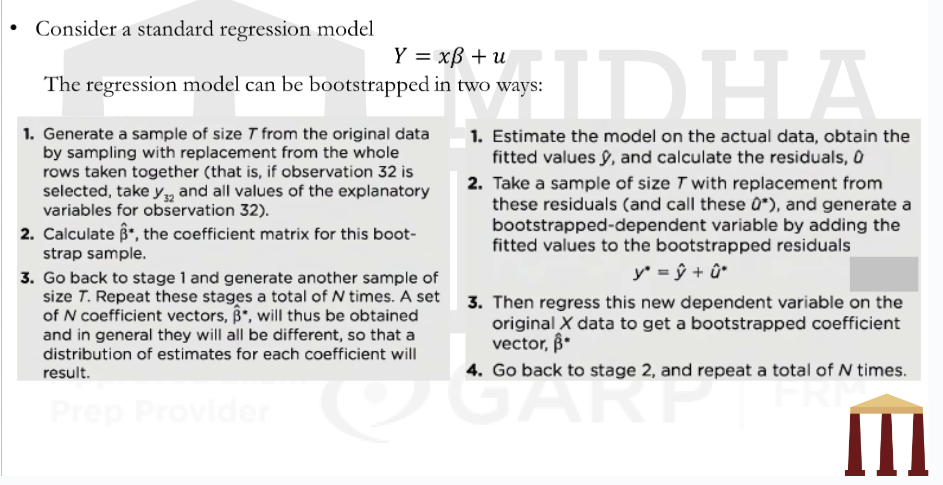
Bootstrapping – example in the context of regression

Ineffectiveness of bootstrapping

• Situations where Bootstrapping is ineffective :

1. Outlier data –  If there are outliers in the data, the conclusions of the bootstrap may be affected. If outliers are taken too frequently (remember it is sampling with replacement) then the representing distribution will have fatter tails and if outliers are not sampled then the distribution will not be a true representative. 
2. Non-Independent data – Bootstrap assumes that the data are independent of one another. However, if there is autocorrelation in the data, then it is not useful. To overcome the same, a method called moving block bootstrap can be used wherein blocks of data are examined at one time in order to preserve the original data dependency.

Random number generation

• The simplest class of number generator are from uniform (0,1) distribution. A uniform distribution is one where values between o and 1 are only chosen with each one having equal chance of being selected. A number generator can be discrete or uniform.

• Recursive process for generating the random number will require the user to specify an initial value to get the process started. The choice of this value will, undesirably, affect the properties of the generated series. This effect will be strongest for y1, y2, . . . , but will gradually die away. For example, if a set of random draws is used to construct a time series that follows a GARCH process, early observations on this series will behave less like the GARCH process required than subsequent data points. Consequently, a good simulation design will allow for this phenomenon by generating more data than are required and then dropping the first few observations. For example, if 1,000 observations are required, 1,200 observations might be generated, with observations 1 to 200 subsequently deleted and 201 to 1,200 used to conduct the analysis.
• These computer-generated random number draws are known as pseudo-random numbers, since they are in fact not random at all, but entirely deterministic, since they have been derived from an exact formula! By carefully choosing the values of the user-adjustable parameters, it is possible to get the pseudo-random number generator to meet all the statistical properties of true random numbers. Eventually, the random number sequences will start to repeat, but this should take a long time to happen. 

Disadvantages of simulation methods

• Computationally intensive

• Results are not precise – The simulation process is based on some assumption about the parameters. However, if there is any error in the assumption in data generating process, it can lead to in accurate results. For example, in the context of option pricing, the option valuations obtained from a simulation will not be accurate if the data generating process assumed normally distributed errors while the actual underlying returns series is fat-tailed.

• Results are hard to replicate – Practically, MCS is not conducted documenting each sequence of random draw and hence results will be specific with each draw. If number of replication is small, a repeat of the experiment would involve different sets of random draws and therefore would be likely to yield different results. 

• Results are experiment specific – Simulation process in finance is based on specific assumptions related to data generating process and set of equations. If the assumptions are changed in
  data generating process or set of equation, the results can be significantly different.

Class exercise 1

• A risk manager was trying to understand on how to reduce the sampling error in MCS. His senior told him about the two methods and asked him to use the most suitable method for his problem.

After going through the research provided by the seniors, the manager made following comment:

1. The manager concluded that the antithetic method will reduce the error due to perfectly negative co-relation between the parameter and its complement while using Asian option valuation.
2. Under control variate technique, the controlled variable has no sampling error.

Which of the following option is correct?

1. I only   
2. II only  
3. I & II both  
4. Neither I nor II

Class exercise 2

• One can not change the assumptions of data generating process or set of equation while implementing MCS . If the above condition is violated, which one of the limitation of MCS it will fall in?

1. High computation cost
2. Results are imprecise 
3. Results are difficult to replicate
4. Results are experiment specific