Measuring Returns

• All estimators of volatility depend on returns, and there are two common methods used to construct returns. The usual definition of a return on an asset bought at time t-1 and sold at time 𝑡 is



where

P_t is the price of the asset in period 𝑡.

• Returns computed using this formula are called simple returns and are traditionally expressed with an uppercase letter (i.e., R_t). The time scale is arbitrary and may be short (e.g., an hour or a day) or long (e.g., a quarter or a year).
• The return of an asset over multiple periods is the product of the simple returns in each period:



• There are also continuously compounded returns, also known as log returns. These are computed as the difference of the natural logarithm of the price:



The log return is traditionally denoted with lower case letter (i.e., r_t).

• The main advantage of log returns is that the total return over multiple periods is just the sum of the single period log returns:



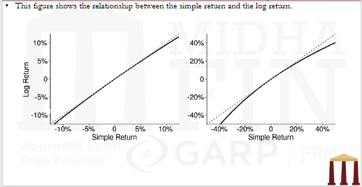
• A log return approximates the simple return. However, the accuracy of this approximation is poor when the simple return is large, and log returns are more commonly used when returns are computed over short time spans.
• Converting between the simple and log return uses the relationship:





• The log return is always less than the simple return. Furthermore, simple returns are also never less than -100% (i.e., a total loss). Log returns do not respect this intuitive boundary and are less than -100%  whenever the simple return is less than -63%.
• The simple additive structure of log returns makes them more attractive in cases where the error is small (i.e., over short periods). For example, it is common for volatility models to use log returns because they are usually computed using daily or weekly data. Despite this common practice, however, it is important to have a sense of the approximation error embedded in log returns when returns are large in magnitude.

Measuring volatility and risk

• The volatility of a financial asset is usually measured by the standard deviation of its returns. A simple but useful model for the return on a financial asset is



where

e_t is a shock with mean zero and variance 1,

μ is the mean of the return (i.e. E[r_t]= μ),and

σ² is the variance of the return (i.e., V[r_t ]=σ²)

• The shock can also be written as:



so that ϵ_t has mean zero and variance σ²

• The shock is assumed to be independent and identically distributed (iid) across observations. While it is not necessary to specify the distribution of e_t, it is assumed that e_t ∼^iid N(0,1). With this assumption, returns are also iid N(μ, σ²). However, while the normal is a convenient distribution to use, it does not provide a full description of most financial returns.
• The volatility of an asset is the standard deviation of the returns (i.e., √(σ^2 )=σ). This measure is the volatility of the returns over the time span where the returns are measured, and so if returns are computed using daily closing prices, this measure is the daily volatility.
• In a simple model, the return over multiple periods is the sum of the returns. For example, if returns are calculated daily, the weekly return is



• The mean of the weekly return is 5μ and, because e_t is an iid sequence, the variance of the weekly return is 5σ² and the volatility of the weekly return is √5σ. Hence,

The mean and the variance scale linearly in the holding period, and

The volatility scales with the square-root of the holding period.

• This scaling law allows the transformation of volatility between time scales. The common practice is to report the annualized volatility, which is the volatility over a year. When the volatility is measured daily, it is common to convert daily volatility to annualized volatility by scaling by √252  so that:



• The scaling actor 252 approximates the number of trading days in the US and most other developed markets. Volatilities computed over other intervals can be easily converted by computing the number of sampling intervals in a year and using this as the scaling factor. For example, if volatility is measured with monthly returns, then the annualized volatility is constructed using a scaling factor of 12:



EXAMPLE –

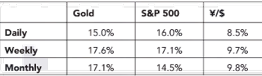
• Consider the volatility of the returns of three assets:
1. Gold (specifically, the price as determined at the London gold fix),
2. The return on the S&P 500 index, and
3. The percentage change in the Japanese yen/US dollar rate (JPY/USD).

Returns are computed daily, weekly (using Thursday closing prices), and monthly (using the final closing price in the month). variance of returns is estimated using the standard estimator:



where

𝜇̂ is the sample average return.

• This table shows the annualized volatilities constructed by transforming the variance estimates. The annualized volatilities are similar within each asset and the minor differences across sampling frequencies can be attributed to estimation error (because these volatilities are all estimates of the true volatility).

Measuring volatility and risk – implied volatility

• Implied volatility is covered in detail in the topic – “Black Scholes Merton Model” in the module – Valuation and Risk Models (VRM)

• The VIX Index is another measure of implied volatility that reflects the implied volatility on the S&P 500 over the next calendar 30 days, constructed using options with a wide range of strike prices. 

• The methodology of the VIX has been extended to many other assets, including other key equity indices, individual stocks, gold, crude oil, and US Treasury bonds. The most important limitation of the VIX is that it can only be computed for assets with large, liquid derivatives markets, and so it is not possible to apply the VIX methodology to most financial assets. Because the VIX Index makes uses of option prices with expiration dates in the future, it is a forward-looking measure of volatility. This differs from backward-looking volatility estimates generated using (historical) asset returns.

The distribution of financial returns

• A normal distribution is symmetric and thin-tailed, and so has no skewness or excess kurtosis. However, many return series are both skewed and fat-tailed.

• For example, consider the returns of gold, the S&P 500, and the JPY/USD exchange rate. All three assets have a skewness that is different from zero and a kurtosis larger than 3. Some important points are –
  • In general, the skewness changes little as the horizon increases from daily to quarterly, whereas the kurtosis declines substantially. 
  • The returns on the S&P 500 and the returns on the JPY/USD exchange rate are both negatively skewed, while the returns on gold are positively skewed. This difference arises because equities and gold tend to move in different directions when markets are stressed -equities decline markedly in stress periods, while gold serves as a flight-to-safety asset and so moves in the opposite direction.

Distribution of returns – jarque bera test

• The Jarque-Bera test statistic is used to formally test whether the sample skewness and kurtosis are compatible with an assumption that the returns are normally distributed.

The null hypothesis in the Jarque-Bera test is



where

𝑆 is the skewness and 𝜅 is the kurtosis of the return distribution. These are the population values for normal random variables.

The alternative hypothesis is



The test statistic is



where

𝑇 is the sample size.

• When returns are normally distributed, the skewness is asymptotically normally distributed with a variance of 6, so that s ̂²/6  has a χ₁²​ distribution. Meanwhile, the kurtosis is asymptotically normally distributed with mean 3 and variance of 24, and so (κ ̂-3)^2/24  also has a χ₁² distribution. These two statistics are asymptotically independent (uncorrelated), and so JB∼χ_2^2.
• Test statistics that have χ^2 distributions should be small when the null hypothesis is true and large values indicate that the null is unlikely to be correct. The critical values of a χ₂²  are 5.99 for a test size (significance level) of 5% and 9.21 for a test size (significance level)of 1%. When the test statistic is above these values, the null that the data are normally distributed is rejected.

EXAMPLE

• Based on a sample of monthly returns for a period of 10 years, a portfolio distribution’s skewness is estimated to 1.05 and kurtosis equal to 4. Test the hypothesis that the fund’s returns follow a normal distribution at a test size of 5%.

Distribution of returns – power laws

• An alternative method to understand the non-normality of financial returns is to study the tails. Normal random variables have thin tails so that the probability of a return larger than 𝑘𝜎 declines rapidly as 𝑘 increases, whereas many other distributions have tails that decline less quickly for large deviations.
• The most important class of these have power law tails, so that the probability of seeing a  realization larger than a given value of 𝑥 is P(X>x)=kx^(-α), where 𝑘 and 𝛼 are constants.
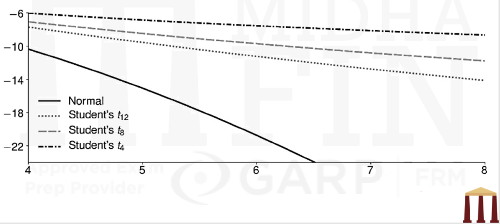
• The Student’s 𝑡 is an example of a widely used distribution with a power law tail.
• The simplest method to compare tail behavior is to examine the natural log of the tail probability. The figure in the next page plots the natural log of the probability that a random variable with mean zero and unit variance appears in its tail [i.e., ln⁡{P r⁡(X>x)}]. Four distributions are shown: a normal and three parameterizations of a Student’s 𝑡.
• The normal curve is quadratic in 𝑥, and its tail quickly diverges from the tails of the other three distributions. The Student’s 𝑡 tails are linear in 𝑥, which reflects the slow decay of the probability in the tail. This slow decline is precisely why these distributions are fat-tailed and produce many more observations that are far from the mean when compared to a normal.

Correlation vs dependence

• The dependence between assets plays a key role in portfolio diversification and tail risk. Two random variables, 𝑋 and 𝑌, are independent if their joint density is equal to the product of their marginal densities:



• Any random variables that are not independent are dependent. Financial assets are highly dependent and exhibit both linear and nonlinear dependence. The linear correlation estimator (also known as Pearson’s correlation) measures linear dependence. Correlation (i.e., 𝜌) and the regression slope (i.e., 𝛽) are related, and the regression slope is zero if and only if the correlation is zero. Regression explains the sense in which correlation measures linear dependence. In the regression



if 𝑌 and 𝑋 are standardized to have unit variance (i.e., σ_X^2=σ_Y^2=1), then the regression slope is the correlation.

• In contrast, nonlinear dependence takes many forms and cannot be summarized by a single statistic. For example, many asset returns have common heteroskedasticity (i.e., the volatility across assets is simultaneously high or low). However, linear correlation does not capture this type of dependence between assets

Correlation measures

• The Pearson approach measures the strength of the linear association between two variables. The Pearson correlation coefficient ρ is defined as



where

X is the set X = {x₁  … , x_n }

Y is the set Y = {y₁, … , y_n}

elements x₁…x_n ∈ R

elements y₁  .. .y_n ∈ R

The covariance in the above equation is defined as



• It has already been discussed in earlier chapters that, for random sets, covariance can also be written as



where

E(X) is the expected value of X

E(Y) is the expected value of Y

E(XY) is the expected value of the product of the random variables X and Y.

We also know that the variances can be defined as



And since standard deviations are square root of the variances, we have



Year	Asset X	Asset Y	Return of Asset X	Return of Asset Y
2008	100	200
2009	120	230	20.00%	15.00%
2010	108	460	-10.00%	100.00%
2011	190	410	75.93%	-10.87%
2012	160	480	-15.79%	17.07%
2013	280	380	75.00%	-20.83%
		Average	29.03%	20.07%

• Even though the application of the Pearson correlation coefficient and the related least squares linear regression analysis is a standard statistical tool in finance, the limitations of the Pearson correlation approach in finance are evident for five reasons:
1. Linear dependencies, are not common in finance. Financial relationships are  typically nonlinear.
2. Zero correlation does not necessarily mean independence. This is because only the first two moments, mean and standard deviation, are considered in the formula of Pearson Correlation. For example, the parabola  Y=X^2 will lead to ρ = 0, which is arguably misleading.
3. Linear correlation measures are natural dependence measures only if the joint distribution of the variables is elliptical. However, only a few distributions such as the multivariate normal distribution and the multivariate Student’s t distribution are special cases of elliptical distributions, for which linear correlation measure can be meaningfully interpreted.
4. The variances of the sets X and Y have to be finite. However, for distributions with strong    kurtosis, for example the Student’s t distribution with v ≤2, the variance is infinite.
5. In contrast to the copula approach, which is invariant to strictly increasing transformations, the Pearson correlation approach is typically not invariant to transformations. For example, the Pearson correlation between pairs X and Y is in general different from the Pearson correlation between the pairs ln⁡(X) and ln⁡(Y). Hence the information value of the Pearson correlation coefficient after data transformation is limited.
• For these reasons, the application of the Pearson correlation concept in finance is questionable. The linear Pearson correlation coefficient can at best serve as an approximation for the typically nonlinear relationship between financial variables.
• The Spearman’s correlation coefficient is sometimes referred to as the Pearson correlation coefficient for ranked variables. It will result in a perfect correlation coefficient of 1 if an increase in the elements x_i is always accompanied by an increase in y_i, regardless of the numerical increase, and vice versa. The Spearman correlation approach is nonparametric in the sense that it can be applied without requiring knowledge of the joint distribution of the variables.
• The following steps are followed to get the Spearman’s rank correlation:
1. The return set pairs of X and Y are ordered with respect to the set X.
2. The ranks of X_i and Y_i are derived.
3. The difference of the ranks are derived as d_i’s
4. The Spearman rank correlation coefficient ρ_s is finally calculated  as

Year	Asset X	Asset Y	Return of Asset X	Return of Asset Y
2008	100	200
2009	120	230	20.00%	15.00%
2010	108	460	-10.00%	100.00%
2011	190	410	75.93%	-10.87%
2012	160	480	-15.79%	17.07%
2013	280	380	75.00%	-20.83%
		Average	29.03%	20.07%

	RANKED RETURN OF Xi	ASSIGNED (SAME YEAR) RETURN OF Yi	RANK OF Xi	RANK OF Yi	di	di2
2012	-15.79%	17.07%
2010	-10.00%	100.00%
2009	20.00%	15.00%
2013	75.00%	-20.83%
2011	75.93%	-10.87%

Correlation vs dependence

• When variables have a linear relationship, rank and linear correlation are usually similar in magnitude. The rank correlation estimator is less efficient than the linear correlation estimator and is commonly used as an additional robustness check.
• Significant differences in the two correlations indicate an important nonlinear relationship. Rank correlation has two distinct advantages over linear correlation.
1. First, it is robust to outliers because only the ranks, not the values of 𝑋 and 𝑌, are used.
2. Second, it is invariant with respect to any monotonic increasing transformation of X_i and Y_i (e.g., X_i  → f(X_i), where f(X_i  ) > f(X_j) when X_i>X_j ). Linear correlation is only invariant with respect to increasing linear transformations (e.g., X_i→ a + bX_i , where b>0). This invariance with respect to a wide class of transformations makes rank correlation particularly useful when examining the relationship between primary and derivative asset returns.

Correlation measures

• Just like Spearman’s correlation coefficient, the Kendall’s τ is ordinal and nonparametric and will result in a perfect correlation coefficient of 1 if an increase in the variable x is always accompanied by an increase in y, regardless of the numerical increase, and vice versa. In most other cases, the two rank correlation measures are not equal.
• Kendall’s 𝜏 measures the relative frequency of concordant and discordant pairs.The Kendall τ is defined as



where n_c  is the number of concordant data pairs and n_d is the number of discordant pairs.

The pair is concordant if x_>x_j and y_i>y_j or x_i<x_j and y_i<y_j  where i≠j

The pair is discordant if x_i>x_j and y_i<y_j or x_i<x_j and y_i>y_j  where i≠j

A pair is neither concordant nor discordant if x_i=x_j or y_i=y_j where i≠j

	RANKED RETURN OF Xi	ASSIGNED (SAME YEAR) RETURN OF Yi	RANK OF Xi	RANK OF Yi
2012	-15.79%	17.07%	1	4
2010	-10.00%	100.00%	2	5
2009	20.00%	15.00%	3	3
2013	75.00%	-20.83%	4	1
2011	75.93%	-10.87%	5	2

	RANKED RETURN OF Xi	ASSIGNED (SAME YEAR) RETURN OF Yi	RANK OF Xi	RANK OF Yi	di	di2
2012	-31.58%	17.07%
2010	-10.00%	100.00%
2009	20.00%	15.00%
2013	75.00%	-20.83%
2011	151.86%	-10.87%

• A special problem with the Kendall τ is when many non-concordant and many non-discordant pairs occur, which are omitted in the calculation. This may lead to only a few concordant and discordant pairs, which can distort the Kendall τ coefficient.

Correlation vs dependence

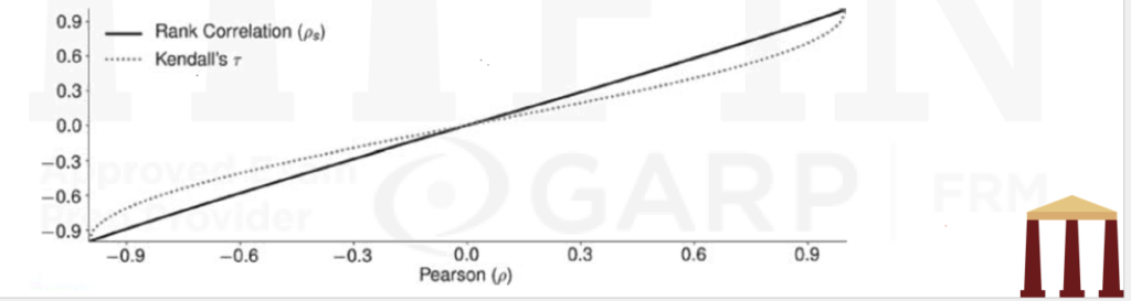
• Kendall’s 𝜏 is the difference between the probability of concordance and the probability of discordance. When all pairs are concordant, then τ ̂  = 1. If all pairs are discordant  τ ̂   is -1. Other patterns produce values between these two extremes. Note that concordance only depends on the pairwise order, not the magnitude of data, and so monotonic increasing transformations also have no effect on Kendall’s 𝜏.
• This figure plots the relationship between linear (Pearson) correlation, rank (Spearman) correlation, and Kendall’s 𝜏 for a bivariate normal.

Structured correlation matrices

• A correlation matrix is interpretable as a covariance matrix where all random variables have unit variance. The fact that any linear combination of random variables must have a non-negative variance imposes restrictions on the values in a correlation matrix of three or more random variables.

For example, suppose that a trivariate normal random variable with components X_1, X_2, and X_3 has mean zero and covariance (and correlation) matrix:

Correlation vs dependence

The variance of an average of the three components:

This value is negative, and so Σ cannot be a valid covariance matrix. This requirement – that any weighted average must have a positive variance, is known as positive definiteness.

• Practitioners commonly impose structure on correlation matrices to ensure that they are positive definite. Two structured correlations are commonly used –
1. The first type sets all correlations equal to the same value (i.e., ρ_ij= ρ ̅ for all pairs 𝑖 and 𝑗), a model known as equicorrelation.
2. The second type uses a factor structure that assumes correlations are due to exposure to a common factor. This type of structured correlation mimics the correlation of assets related through CAPM, so that the correlation between any two entries can be written as ρ_ij= γ_i γ_j  , where both γ₁ and γ₂ are between -1 and 1.