Introduction

• Covariance-stationary time series have mean, variance, and autocovariances that do not depend on time. Any time series that is not covariance-stationary is non-stationary. Three most pervasive sources of non-stationarity in financial and economic time series are –

1. Time trends – Time trend models capture the propensity of many time series to grow over time. These models are often applied to log transformation to capture the growth rate. Estimation of parameters in trend models that contain no other dynamics are simple.

2. Seasonality – It induces non-stationary behavior in time series by relating the mean of the process to the month or quarter of the year. It can be modeled in one of two ways –
   1. Shifts in the mean that depend on the period of the year.
   2. An annual cycle where the value in the current period depends on the shock in the same period in the previous year. 

Two approaches to model seasonal time series are –

1. Using dummy variables for month or quarter
2. Using the year-over-year change in the variable to eliminate the seasonality in the transformed data series
3. Unit root(random walk) – This is the most pervasive form of non-stationary in financial and economic time series. A time series that follows a random walk depends equally on all past shocks. Directly modeling such time series is difficult because parameter estimators are biased and are not normally distributed , even in large samples. the solution to this is that, instead of modeling the data, their difference should be modelled(y_t -y_t-1).

Time Trends

• Non-stationary time series may have trends which can be deterministic, stochastic or both. If the trends are stochastic, it is treated differently as it contains unit root. On the other hand, deterministic trends can be modelled using time trend models. A time trend deterministically shifts the mean of a series. Some common time trend models are –
  • Linear trend models
  • Quadratic trend models
  • Logarithmic Trend Models –
    1. Log-linear trend models
    2. Log-quadratic trend models

Time Trends – linear trends

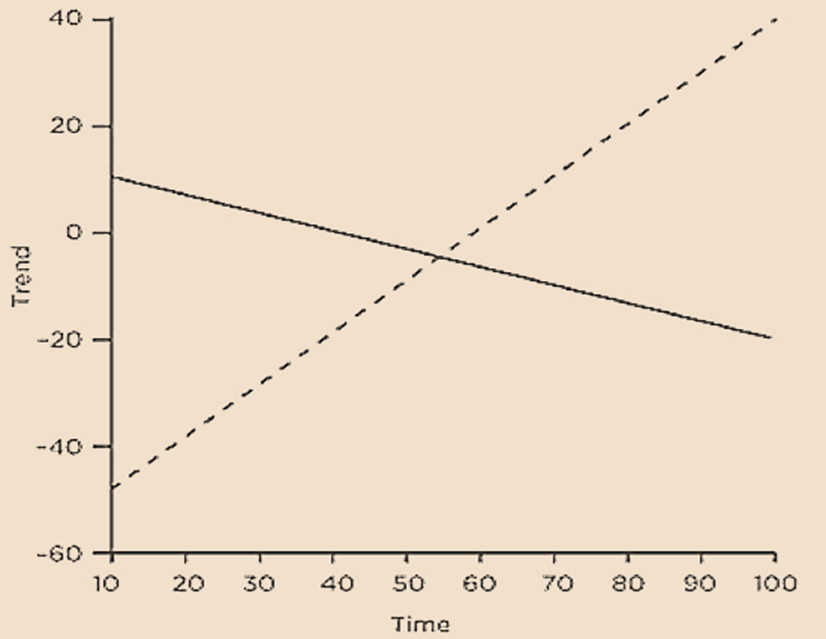
• The most basic type of non-stationary time series is a process with a linear time trend. If a variable changes at a constant rate, then the variable is said to exhibit linear trend. Linear trend can be increasing or decreasing and can be expressed as –



where



• This process is non-stationary because the mean depends on time –



where,

the time trend δ_1 measures the average change in 𝑌 across subsequent observations.

• This figure shows two linear trends – increasing linear trend (depicted by dashed line) and decreasing linear trend (depicted by solid line).



• A linear trend model implies that the series grows by a constant quantity each period. In economic and financial time series, this is problematic for two reasons –

If the trend is positive, then the growth rate of the series will fall over time.

If slope coefficient is less than zero, then Y_t will eventually become negative. However, this is not plausible for many financial time series (e.g., prices or quantities).

Time Trends – Quadratic Trends

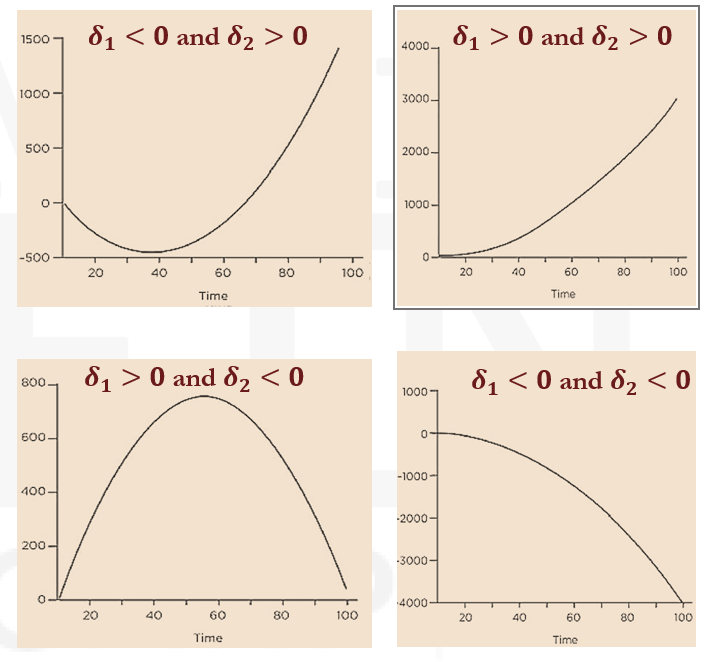
• Quadratic trends are used to provide local approximations. Quadratic trend models can potentially capture non-linearities in trends.  This can be expressed as –



• A variety of different non-linear quadratic trend shapes are possible, depending on the signs of the coefficients δ₁ and δ₂.

If δ₁>0 and δ₂>0, the trend is monotonically, but nonlinearly, increasing

If δ₁<0 and δ₂<0 , the trend is monotonically, but nonlinearly decreasing.

If δ₁<0 and δ₂>0, the trend has a U shape

If δ₁>0 and δ₂<0 , the trend has an inverted U shape.



• Trend model can be generalized to a polynomial time trend model by including higher powers of time. This is expressed as –



In practice, most time trend models are limited to first (i.e., linear) or second-degree (i.e., quadratic) polynomials.

• The parameters of a polynomial time trend model can be consistently estimated using OLS. The resulting estimators are asymptotically normally distributed.
1. Standard errors and 𝑡-statistics can be used to test hypotheses only if the residuals are white noise.
2. If the residuals are not compatible with the white noise assumption, then the 𝑡-statistics and model R² are misleading.

Time trends – logarithmic trends

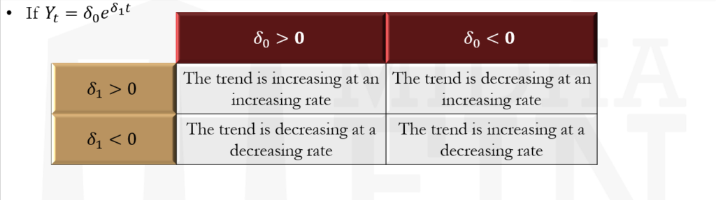
• Most financial and macroeconomic variables might change at an increasing or decreasing rate rather than at a constant rate which happens in linear trends. This can imply that the trend itself changes at a constant (or non-constant) growth rates.
• Constant growth rates in trends can be examined using a log-linear models that relate the natural log of Y_t to a linear trend. If trend is characterized by constant growth rate δ_1, then it can be expressed as –



This trend is non-linear function of time in levels, but the logarithmic transformation of this relationship can be expressed as –



where

ln⁡Y_t is a linear function of time.

• This model implies that:



so that the growth rate of 𝑌 is constant.



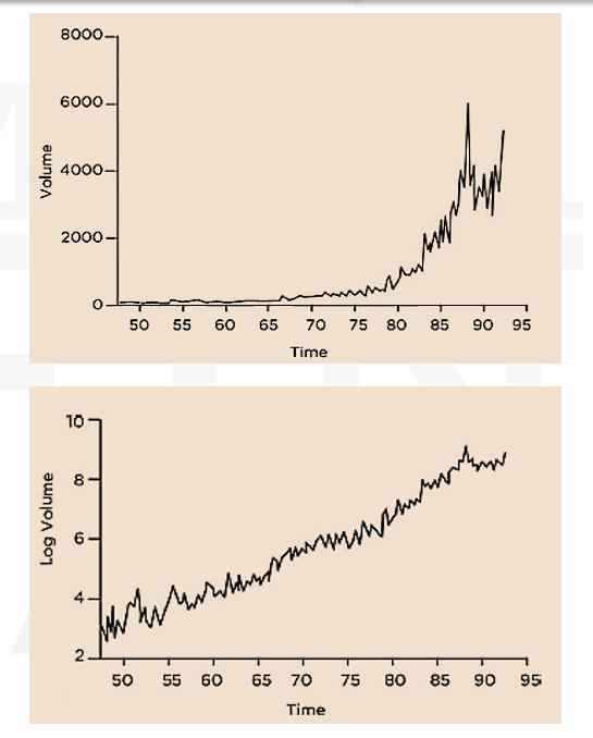
• This figure shows the –



1. monthly volume of shares traded on the NYSE (upper panel), and
2. logarithm of monthly volume of shares traded.

The logarithmic trend is approximately linear.

• Log-linear models can be extended to higher powers of time. For example, the log-quadratic time trend model can be expressed as –



This expression implies that the growth rate of Y_t  is δ₁+2δ₂ t, and so depends on time.

• In practice, log-linear models are sufficient to capture the trend in series that grow over time.

Seasonality

• A seasonal pattern is one that repeats itself every year. The annual repetition can be exact (deterministic seasonality), or approximate (stochastic seasonality). 

• Seasonality appears in financial and economic time series. Some common examples of seasonality that occur in financial market are –

1. The January effect – It posits that equity market returns are larger in January than they are in the other months of the year. 

2. Calendar effects – It generalizes seasonality to cycles that do not necessarily span an entire year. For example, an anomaly has been identified where Monday returns are statistically significantly lower than Friday returns in US equity data. Calendar effects also appear in intra daily data, where trading volume and price volatility follow a “U” shaped pattern of spikes during the market  opening/closing and a mid-day lull.

Seasonality – seasonal dummy variables

• Deterministic seasonality produces differences in the mean of a time series that are simple to model using dummy variables. If it is Supposed that Y_t is a purely seasonal time series that has a different mean in each period and repeats after every 𝑠 periods (e.g., every four in a quarterly series or 12 in a monthly series), it can be modeled as –



where,



The function a (mod b) yields the remainder of (a/b). For example, 10 (mod 6)=4.

It should be noted that dummy variable I_st has been omitted to avoid the dummy variable trap, which occurs when dummy variables are multicollinear.

• The mean of each period for the above-mentioned seasonal model is given as –
1. The mean in period 1 is E[Y₁ ]= δ+γ₁
2. The mean in period 2 is E[Y₂ ]= δ + γ₂
3. The mean in period 𝑠 is E[Y_s]=δ because all dummy variables are zero.

Seasonality

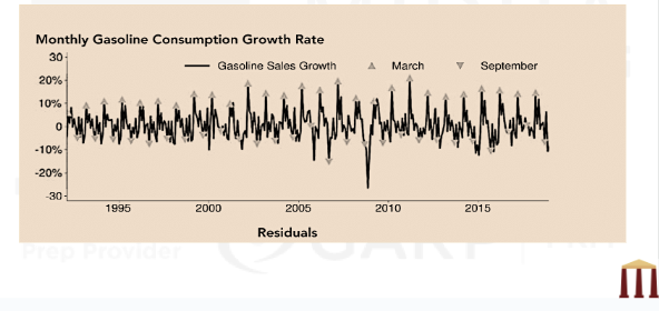
• The parameters of this model are estimated  using OLS by regressing Y_t on a constant and s-1 dummy variables. 𝛿 is interpreted as the average of Y_t in period 𝑠, whereas γ_j measures the difference between the period 𝑗 mean and the period 𝑠 mean.
• This figure gives an example where the seasonality pattern in monthly gasoline consumption growth rate has been shown.

Time trends, seasonalities, and cycles

• Deterministic terms (e.g., time trends and seasonalities) are often insufficient to describe economic time series. As a result, the residuals from models that only contain deterministic terms tend not to be white noise. When the residuals are not white noise but appear to be covariance-stationary, then the deterministic terms can be combined with AR or MA terms to capture the three components of a time series –

the trend, the seasonality, and the cyclicality.

• Suppose a trend model is given as –



Adding AR terms and seasonal dummies will produce a model which can be expressed as –



where

δ₁ captures the long-term trend of the process,

γ_i measure seasonal shifts in the mean from the trend growth (i.e., δ₁ t), and

ϕY_(t-1) is an AR term that captures the cyclical component.

• A process is trend-stationary if removing a deterministic time trend produces a series that is covariance-stationary. While adding a cyclical component is a simple method to account for serial correlation in trend stationary data, many trending economic time series are not trend-stationary. 

• If a series contains a unit root (i.e., a random walk component), then detrending cannot eliminate the non-stationarity.

• Adding and/or combining terms in the time series may not always result in the model which is appropriate. Sometimes, for example, the Ljung-Box test statistics might imply rejecting the null hypothesis.

random walks and unit roots

• Random walks and their generalization, unit root processes, are the third and most important source of non-stationarity. A simple random walk process evolves according to –



Using the above, substituting t-1 in place of t, Y_(t-1) will be equal to Y_(t-2)+ϵ_(t-1). Substituting this value of Y_(t-1)  into the above random walk, the model can be expressed as –



If the substitution is repeated until observation zero is reached, the above model can be expressed as –



This shows that Y_t depends equally on all shocks between periods 1 and 𝑡, and on an initial value Y₀.

• Random walks place equal weight on all shocks and the initial value, and so a shock in period 𝑡 permanently affects all future values.
• Unlike covariance-stationary time series, which always mean revert, random walks become more dispersed over time. The variance of a random walk is V[Y_t ]=tσ^2. Since they are not covariance stationary, they cannot be modeled directly by AR, MA, or ARMA models.
• Unit roots generalize random walks by adding short-run stationary dynamics to the long-run random walk. A unit root process is usually described using a lag polynomial as –



where

ϵ_t∼ WN(0, σ²) is a white noise process, and

θ(L) ϵ_t  is an MA.

• For example, suppose an AR(2) process is expressed as –



It can be written with a lag polynomial as:



The unit root is evident in the factored polynomial.

The problems with unit roots

• Three key challenges when modeling a time series that has a unit root are –
1. Dickey-Fuller (DF) distribution – Parameter estimators in ARMA models fitted to time series containing a unit root have Dickey-Fuller (DF) distribution. The DF distribution is asymmetric, sample-size dependent, and its critical values depend on whether the model includes time trends. These features make it difficult to perform inference and model selection when fitting models on time series that contain unit roots.
2. Spurious relationships – A pair of time series have spurious relationship when there are no fundamental links between them, but a regression of one on the other produces a coefficient estimate that is large and seemingly statistically different from zero. When a time series contains a unit root, it is common to find spurious relationships with other time series that have a time trend or a unit root.
3. A unit root process does not mean revert. Mean-reversion affects the forecasts of stationary AR models so that E_t [Y_(t+h) ]≈E[Y_t] when ℎ is large. But a random walk is not stationary and E_t [Y_(t+h)]=Y_t for any horizon ℎ.
• The solution to all three problems is to difference a time series that contains a unit root. If Y_t has a unit root, then the difference, ΔY_t  (Y_t-Y_(t-1) ) does not have unit root.
• Suppose a random walk process is expressed as –



The difference of this process will not contain unit root. This can be shown as –



Hence, ΔY_t is a constant plus a white noise shock.

• Another interpretation can be made from the general case of a unit root process which can be expressed as –





In this process, since 𝜙(𝐿) is a lag polynomial of a stationary process, the random variable defined by the difference (i.e., ΔY_t) must be stationary.

Testing for unit roots

• Unit root tests examine whether the process contains a unit root. They can also distinguish trend-stationary models from unit root processes with drift.



• The ADF test statistic is the 𝑡-statistic of γ ̂ (i.e. the estimate of γ).
• Implementing an ADF test on a time series requires making following two choices –
1. which deterministic terms to include
2. the number of lags of the differenced data to use

The number of lags to include is simple to determine. It should be large enough to absorb
any short-run dynamics in the difference ΔY_t. The lagged differences in the ADF test are included to ensure that ϵ ̂_t  is a white noise process. The recommended method to select the number of lagged differences is to choose the lag length that minimizes AIC because AIC tends to select a larger model than other criteria such as the BIC. Selecting too many lags is better than selecting too few.

The included deterministic terms have a more significant impact on the ADF test statistic. The DF distribution depends on the choice of deterministic terms.

1. Including more deterministic terms skews the distribution to the left, and so the critical value becomes more negative as additional deterministic terms are included. This makes rejecting the null more difficult when a time series does not contain a unit root, and hence the power of the ADF test is reduced. Therefore, all relevant deterministic terms should be included.
2. The recommended method is to include any deterministic regressor that is statistically significant at the 10% level. If the trend is insignificant at the 10% level, then it can be dropped, and the ADF test can be re-run including only a constant. If the constant is also insignificant, then it too can be dropped, and the test is re-run with no deterministic components. However, most applications to financial and macroeconomic time series require the constant to be included.
• In general, the steps that should be followed to test for unit roots are as follows –
1. Appropriate number of deterministic terms and lagged differences are selected for the ADF regression.
2. One-sided null hypothesis is tested.

H₀:γ=0 (time series is random walk)

H_A:γ<0 (time series is covariance stationary), where γ is the coefficient of lagged level.

3. If the null cannot be rejected, then the series should be differenced because it suggests that the series is non-stationary.
4. The ADF test is repeated for differenced series. If this also non-stationary (null cannot be rejected), the series should be differenced again (double differencing).
5. If the double differenced series is also non-stationary, then the series should be transformed.

Testing for unit roots – result example

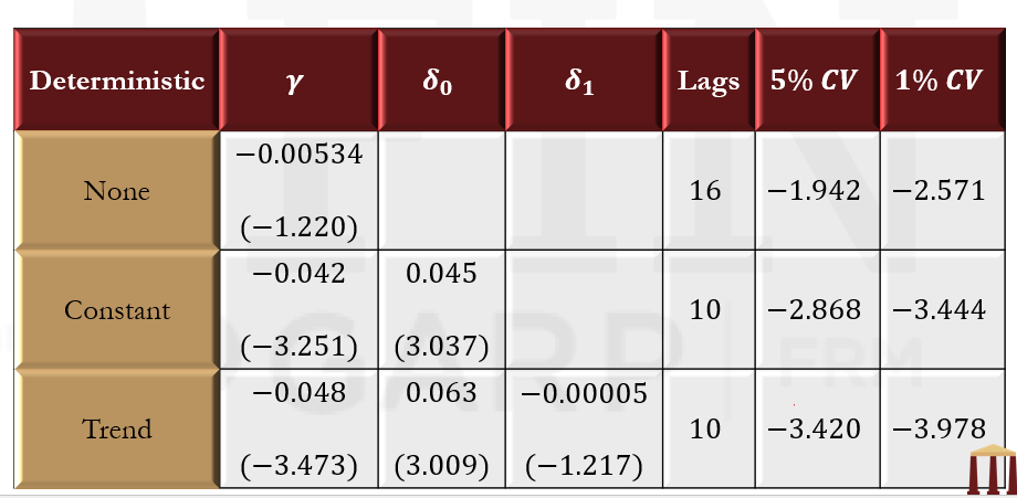
• This table shows ADF test results for the default premium, defined as the difference between the interest rates on portfolios of Aaa-Rated and Baa-Rated bonds. The column γ reports the parameter estimate from the ADF and the ADF statistic in parentheses. The columns δ₀ and δ₁ report estimates of the constant and linear trend along with t-Statistics. The lags column reports the number of lags in the ADF regression as selected by the AIC. The final columns report the 5% and 1% critical values.

Seasonal differencing

• Seasonal differencing is an alternative approach to modeling seasonal time series with unit roots. The seasonal difference is constructed by subtracting the value in the same period in the previous year. This transformation eliminates deterministic seasonalities, time trends, and unit roots.
• By removing trends, seasonality, and unit roots, seasonal differencing produces a time series that is covariance  stationary. The seasonally differenced time series can then be modeled using standard ARMA models. Seasonally differenced series are directly interpretable as the year-over-year change in Y_t or as the year-over-year growth rate in Y_t(when logarithmic transformation of Y_t is considered).
• Many financial and economic time series are highly persistent but stationary, and differencing is only required when a time series contains a unit root. When a time series cannot be easily categorized as stationary or non-stationary, it is good practice to build models for the series in both levels and differences.

Spurious regression

• Spurious regression is a common pitfall when modeling the relationship between two or more non-stationary time series.
• Spurious regression is a frequently occurring problem when both the dependent and one or more independent variables are non-stationary. Since, it is not an issue in stationary time series, so ensuring that both X_t and Y_t are stationary (and differencing if not) prevents this problem.

Forecasting – time trends

• Constructing forecasts from models with time trends, seasonalities, and cyclical components is no different from constructing forecasts from stationary ARMA models. The forecast is the expected value of Y_(T+h) at time T. For example, suppose a linear time trend model is –



• Y_(T+h) for this model can be found as –



• The expectation of Y_(T+h) at time 𝑇 will be –

Forecasting – seasonality

• Forecasting seasonal time series in models with dummies requires tracking the period of the forecast. If the dummy-only model for data with a period of 𝑠 is given as –



The ℎ-step ahead forecasts are constructed as



where j=(T+h) (mod s).

Forecasting – confidence intervals

• When the error is Gaussian white noise N(0, σ^2), then the 95% confidence interval for the future value is given as –



• In practice, 𝜎 is not known. However, it can be estimated as the square root of the residual variance from the estimated regression.
• Confidence intervals can be constructed for forecasts from any model, whether the process is stationary or not.
• The confidence interval only depends on the variance of Y_(T+h)– E_T [Y_T+h].